SafeRevert: When Can Breaking Changes be Automatically Reverted?
Tim A. D. Henderson, Avi Kondareddy, Sushmita Azad, and Eric Nickell.
SafeRevert: When Can Breaking Changes be Automatically Reverted?. ICST Industry Track 2024.
DOI.
PDF.
WEB.
Note
This is a conversion from a latex paper I wrote. If you want all formatting correct you should read the pdf version.
Abstract
When bugs or defects are introduced into a large scale software repository, they reduce productivity. Programmers working on related areas of the code will encounter test failures, compile breakages, or other anomalous behavior. On encountering these issues, they will need to troubleshoot and determine that their changes were not the cause of the error and that another change is at fault. They must then find that change and revert it to return the repository to a healthy state. In the past, our group has identified ways to identify the root cause (or culprit) change that introduced a test failure even when the test is flaky. This paper focuses on a related issue: at what point does the Continuous Integration system have enough evidence to support automatically reverting a change? We will motivate the problem, provide several methods to address it, and empirically evaluate our solution on a large set (25,137) of real-world breaking changes that occurred at Google. SafeRevert improved recall (number of changes recommend for reversion) by 2x over the baseline method while meeting our safety criterion.
Introduction
Large scale software development is enabled by automatically executing tests in a continuous integration environment. Continuous integration (CI) (Fowler 2006) is the industrial practice of using automated systems to automatically integrate changes into the source of truth for the software system or repository. This improves collaboration by helping software developers avoid breaking compilation, tests, or structure of the system that others are relying on.
Corporations and teams may engage in CI using adhoc tools across many independent software repositories. For instance Github (github.com) supports CI “Actions" which can be integrated into any repository. However, many organizations are recognizing the value of using a “mono-repository" (monorepo) development model where many or all teams in the organization use a single shared software repository (Potvin and Levenberg 2016). At the largest organizations such as Google (Potvin and Levenberg 2016; Memon et al. 2017; Henderson et al. 2023), Microsoft (Herzig and Nagappan 2015), and Facebook (Machalica et al. 2019) large repositories are complimented by advanced centralized CI systems.
In these large, modern CI systems, the integration goes beyond just ensuring the code textually merges. Compilations are invoked, tests are executed, and additional static and dynamic verification steps are performed. The demand for machine resources can exceed capacity for build, test, and verification tasks desired by a large-scale CI system. To combat this problem, test case selection or prioritization is used (Gupta, Ivey, and Penix 2011; Micco 2013; Machalica et al. 2019) to select fewer tests to run.
Additionally, CI steps are often invoked at multiple points in the Software Development Life Cycle. In the past, it may have been assumed that the tests were executed by the CI system once, at the time a commit was created in the version control. Today, CI may execute tests multiple times during development: when a change is sent for code review, immediately prior to submission or integration into the main development branch, after one or more changes has been integrated into the development branch, and when a new release is created. This paper is primary concerned with testing that occurs after the code has been integrated into the main development branch.
Why is Testing Necessary After Code Integration?
When deploying CI for the first time, many organizations primarily focus on conducting testing at the time a change is merged into the main branch. For instance, they may test when a Pull Request (PR) on Github is going to be merged into the main branch. The PR is merged if the tests pass and no changes have been made to the main branch since the testing started. This strategy works well until the rate of PR submission exceeds the average amount of time it takes to run all the tests.
At this point, organizations may do a stop gap fix such as adding more machines to run tests in parallel or reducing the size of the test suite. However, at some point, these measures will prove ineffective and the rate that testing can be conducted will become a impediment to an organization’s engineering velocity. To address this, one common solution is to introduce a “submission queue" which batches changes together for testing and merges them all if the tests pass (Ananthanarayanan et al. 2019). If the tests fail, the offending change must be identified and the remaining changes in the batch must be retested (at least doubling the total testing time) (Najafi, Shang, and Rigby 2019).
As the submission rate continues to increase, the organization may add conservative test selection based on file-level dependence analysis (Ananthanarayanan et al. 2019). But at this point, the organization will be reaching the limit of what can be done to completely prevent any breaking changes from being integrated into the main development branch beyond just buying more and more machines to further parallelize the testing.
And what about just buying more machines? Won’t this effectively solve the problem? It would until the submission rate exceeds the time it takes to run the slowest test. At this point, the number of machines purchased can only partially control impact to developer productivity. Even with a very large budget for testing, the number of changes per batch will continue to grow as increases in the number of machines will not reduce the batch size but only keep the testing time per batch relatively constant. The larger the batch size, the more likely that a developer will experience conflicts with another change when attempting to submit. These conflicts (either at the syntactical or semantic level) will make it difficult for developers to reliably submit their changes and require them to constantly monitor the submission process. This monitoring will hurt overall developer productivity.
At the highest submission rates seen in industry today, using submission queues that guarantee zero breaking changes becomes infeasible both from a machine cost perspective and from a developer productivity perspective. Therefore, many organizations relax the requirement that an integrated change will never break a test. Even while using submit queues to gate contributions for a single team, Google has relied on postsubmit testing for mission-critical software since the early 2000s as documented by Mike Bland (Bland 2012).
Post Submission Testing
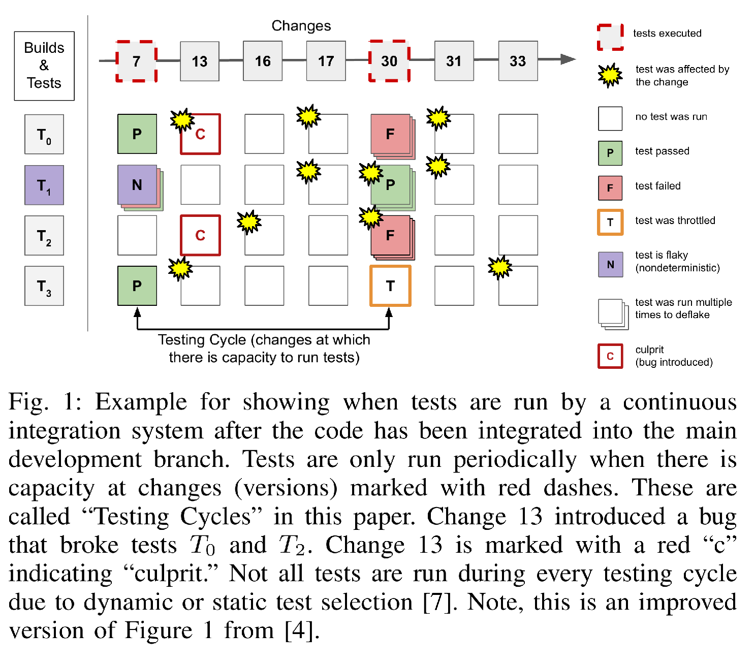
The purpose of testing after a change has been integrated (called Post-Submission Testing or Postsubmit Testing hereafter) is to identify defects that slipped through testing that occurred prior to integration. Typically, organizations are unable to run all tests at every integrated change. Instead, testing is conducted periodically. In this paper we will refer to this periodic testing as Testing Cycles.
Figure [fig:ci-timeline] is a simplified view of the postsubmit testing strategy used at Google. The test scheduler waits until our Build System (Wang et al. 2020) has capacity to start a test cycle. It then schedules tests and then waits until the system has capacity again. When scheduling tests, certain tests may be temporarily skipped or throttled to conserve resources. As shown in Figure [fig:ci-timeline], this leads to the system usually detecting new failures some time after the version that introduced them had been integrated. This leads to the problem of “Culprit Finding."
Culprit Finding
Culprit finding is conceptually simple: given a list of versions that may have introduced a fault, locate the offending change. One may solve this problem with a variety of techniques: Zeller’s Delta Debugging (Zeller 1999), Git’s bisection algorithm (Couder 2008), or Google’s Flake Aware Culprit Finding (FACF) algorithm (Henderson et al. 2023). Every technique used to identify the offending change will have some error rate in industrial practice.
But wait! How can a binary search or delta debugging have an “error rate"? The answer is that old nemesis of industrial practice: flaky or non-deterministic test behavior (Parry et al. 2022). Flaky tests can be caused both by problems in the production code (ex: race conditions causing rare errors), in the test code (ex: use of “sleep") and by infrastructure problems (ex: unreliable machine with bad ram or network congestion). All of these problems behave in version non-hermetic ways, where failures may not be strictly linked to the version of code executed. Furthermore, even when the test is fully version hermetic the flakiness may not obey a Bernoulli distribution as subsequent executions may not be fully independent of the prior ones.
The above issues mean that even culprit finding algorithms such as FACF (Henderson et al. 2023) that have been purpose-built to mitigate flakiness will have some error rate. While that error rate will be much less than a naive algorithm, it may still be high enough to cause problems when deployed in certain environments.
Automatically Reverting Changes
Once an organization has a reliable and high performance culprit finding system, it is natural to use it to automatically revert (undo, roll back) changes that introduce defects into the main development branch. By automatically undoing these changes, the system decreases the amount of time developers working with impacted tests will experience breakages that are unrelated to the changes they are working on. It will also increase the number of versions that are viable to be used to make software releases. Reducing development friction and increasing the number of release candidates improves developer productivity by reducing the amount of time developers spend troubleshooting tests that were broken by someone else.
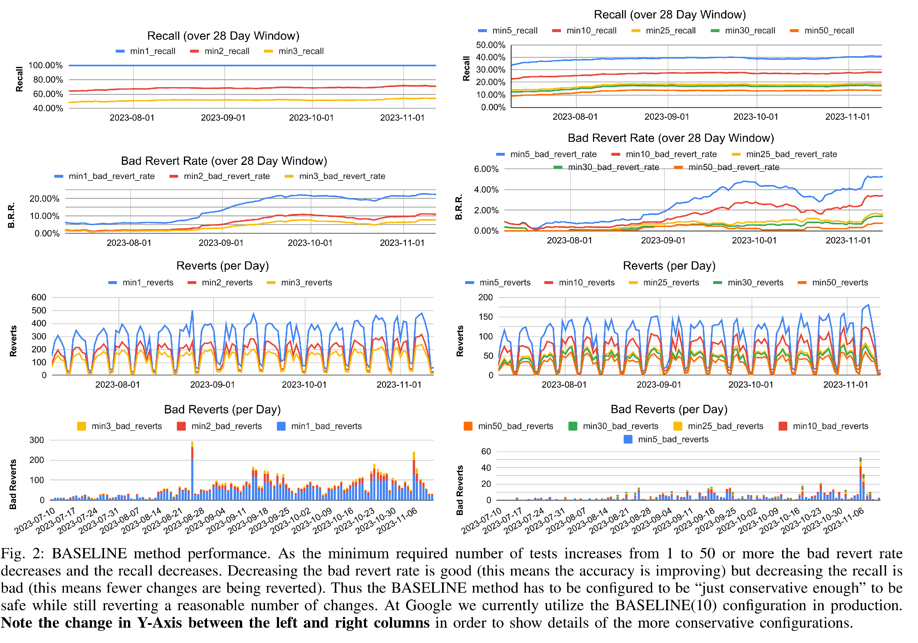
Unfortunately, naively integrating FACF directly into a system that immediately reverts all changes it identifies will lead to unhappy developers. This is because even though Google’s FACF has a measured per-test accuracy of 99.54%, when aggregated (grouped) by blamed change, the accuracy per-change is only 77.37% in the last 28 day window as of this writing.1 This would translate into incorrectly reverting approximately 20-130 changes per day out of an approximately of 300-500 total changes per day reverted (see Figure [fig:baseline]). At Google, we find the cost of incorrectly reverting a change is extremely high in terms of developer toil and frustration. Therefore, we need to reduce the rate of bad reversions as much as possible. In this work, we aim to incorrectly revert fewer than one change per day on average.
Our Contributions and Findings
In this paper we propose a shallow machine-learning based method for using the output of a culprit finding algorithm to automatically revert (undo, rollback) a change that controls for potential errors from the culprit finding algorithm. Our method is generic and can be used with any culprit finding algorithm.
SafeRevert: a method for using the output of any culprit finding algorithm to automatically revert (undo) a change. SafeRevert controls for the error rate while increasing total number of reversions over baseline methods.
An ablation study on the models, designs and features used by the machine learning system used in SafeRevert to identify the most impactful features and best models.
A large scale study on SafeRevert’s efficacy using \(\thicksim\)25,137 potential culprit changes identified by Google’s production culprit finder over a \(\sim\)3 month window yields a recall of 55.7%, \(\sim2.1 \times\) higher than the baseline method.
Background
The Test Automation Platform (TAP) is a proprietary Continuous Integration (CI) system at Google. It runs tests that execute on a single machine without the use of the network or external resources.2 All tests on TAP are required to run in under 15 minutes and exceeding that limit is considered a test failure. TAP executes tests both before a user submits their changes and after the user has submitted their change. This paper is only concerned with the testing that has occurred after a user has submitted a change. At Google, this is referred to as “Postsubmit Testing". The part of TAP that does Postsubmit Testing is called TAP Postsubmit.
TAP has appeared in the literature several times (Gupta, Ivey, and Penix 2011; Micco 2012, 2013; Memon et al. 2017; Leong et al. 2019; Wang et al. 2020; Henderson et al. 2023) and there has been gradual evolution its testing strategy over the years. However, in general TAP uses a combination of static and dynamic Test Selection, execution throttling, and just-in-time scheduling to control testing load. A simplified diagram of TAP Postsubmit testing is visualized in Figure [fig:ci-timeline]. Tests are periodically run in Testing Cycles.3 During a cycle, Projects that are eligible to run their test in the cycle are selected. Tests from those projects are included if some file was modified since that test’s last execution can influence their behavior via inspection of a dependence graph at the Build Target and File level granularity (Gupta, Ivey, and Penix 2011; Micco 2012). When breakages inevitably occur culprit finding is conducted using the FACF algorithm to locate the offending change (Henderson et al. 2023).
FACF operates on a single test target at a time. For simplicity, we use the term “test” both for a target which executes test code or for a “build targets” which verifies that a binary can compile. Conceptually, FACF performs a “Noisy Binary Search” (Rivest, Meyer, and Kleitman 1978) (also called a Rényi-Ulam game (Pelc 2002)) which FACF models under the Bayesian Search Framework (Ben-Or and Hassidim 2008). The input to FACF includes the suspect changes (“suspects”) that may have broken the test and an estimate collected by an independent system of how likely it is to fail non-deterministically without the presence of a deterministic bug, it’s “flakiness”. Much like a normal binary search, it then divides the search space, executes tests, and updates a probability distribution based on the outcomes. Eventually, the system will determine that one of the suspects is above a set probability threshold (.9999) and is the source of the test failure, or that none of the suspects is at fault and the original failure was spurious, due to a flake (non-deterministic failure).
Culprit Finding Accuracy
Now some caveats: The math behind FACF (Henderson et al. 2023) assumes that individual test executions of the same test at either the same version or different versions are independent statistical events. That is, a prior or concurrent execution of a test cannot influence a subsequent execution. Unfortunately, while this assumption is theoretically sound, in practice this property does not always hold. External factors outside a program’s code can also influence a test’s execution behavior. For example, the time of day, day of year, load on the machine, etc., can all influence the outcome of certain tests. Thus, while we have configured FACF to have an accuracy of 99.99%, in practice we do not observe this level of accuracy. As noted in the Introduction, our observed accuracy was 99.54% in the last 28 day window as of this writing. This level of accuracy is consistent with the empirical study conducted in the 2023 paper (Henderson et al. 2023).
How was accuracy “observed”? What was the ground truth used? By what measurement technique? At Google, we continuously randomly sample a subset of culprit finding execution results as they are completed. The selected sample is then cross checked by performing extensive reruns that demand a higher level of accuracy and assume a worse flakiness rate for the test than used for culprit finding. Additionally, more reruns are scheduled for a later time to control for time-based effects. Finally, execution ordering effects are controlled for by ensuring that executions at versions that should fail can fail both before and after versions that should pass are executed. Full details on our methods for verification can be found in the FACF paper (Henderson et al. 2023). Even with extensive reruns there remains a small probability of error. While our method of verification is imperfect, it allows for continuously computing a statistical estimate on the accuracy of the culprit finder.
Measurements of FACF accuracy reported in the 2023 paper were performed per test breakage. That is, culprit finding is performed on a test \(t\) when it has an observed failure at some version \(\beta\) when it was previously passing at a prior version \(\alpha\). The range \((\alpha, \beta]\) is referred to as the search-range and the key \(\{t \times (\alpha, \beta]\}\) is the search-key. For a given search-key, the culprit finder first filters the search-range to changes on which \(t\) has a transitive build dependence, which we call the suspect-set. A culprit \(\kappa\) is identified somewhere between \(\beta\) and \(\alpha\) (e.g. \(\alpha \sqsubset \kappa \sqsubseteq \beta\) where \(a \sqsubset b\) indicates version \(a\) is before version \(b\)). It is possible that there are multiple \(\kappa_t\) for different \(t\) w.r.t. the same search range, which we can call the culprit-set of the search range. What is measured is whether or not \(\kappa\) is correct (true or false) for a given \(t\) and search range \(\alpha \sqsubset \beta\). Accuracy is the total correct measurements over the total number of measurements taken.
Applying Culprit Finding Results to Change Reversion
When breaking changes get merged into the main development branch they impede development productivity. At Google we term impediments to productivity as “friction.” Breaking changes impact three types of friction tracked at Google: Release Friction, Presubmit Friction and Development Friction. Release Friction occurs when breaking changes that merge into the main development branch impede automated releases and require manual intervention by the primary team’s on-duty engineer. Presubmit Friction occurs when pre-submission (“presubmit”) testing in TAP fails due to a broken test in the main development branch. Development Friction occurs when a developer manually triggers the execution of a test broken on the main branch during active code development. All three types of friction can steal time from developers and reduce productivity.
To reduce friction, changes that break tests can be automatically reverted (“rolled back”). However, auto-revert (“auto-rollback”) only improves developer productivity if the changes reverted actually broke tests. Let’s consider for a moment what happens when a change is incorrectly reverted. The developer who authored the change now needs to go on a wholly different troubleshooting journey to determine why their change didn’t stay submitted, and they are faced with the same damning-but-incorrect evidence used to revert their change. The developer is frustrated and must now debug tests that their team doesn’t own and which their changes should not affect.
Some changes are particularly difficult to submit with a buggy auto-revert system: those that change core libraries. These changes have the potential to break a large number of tests and impact a large number of other developers. But, at the same time they are also more likely to be incorrectly blamed (as TAP tracks what tests are affected by each change and uses this as an input to culprit finding). Past auto-revert systems that have been too inaccurate have caused core library authors to opt their changes out of auto reversion as the productivity cost to the core library teams has been too great to bear.
Accuracy of Auto-Revert versus Culprit Finding
A change \(\kappa\) that breaks a test may have broken more than one. If so, then multiple independent executions of the culprit finding algorithm (one for each broken test) will blame the version \(\kappa\) as the culprit. As explored above, the algorithms have an error rate. A change \(\kappa\) that breaks \(n\) tests will have \(m \le n\) culprit finding conclusions that correctly identify \(\kappa\) as the culprit.
Our concern with auto-revert isn’t the accuracy of culprit finding per search-key \(\{t \times (\alpha, \beta]\}\) but rather per culprit change \(\kappa\). Let \(K\) be the set of all changes in the repository blamed as culprits by the culprit finding system. Let \(c \subseteq K\) be the subset of the culprits that are correct and \(\overline{c} \subseteq K\) be the subset of culprits that are incorrect. Then if every culprit in \(K\) was automatically reverted, the accuracy of the auto-revert system would be \({\left|{c}\right|} / {\left|{K}\right|}\). In the introduction, we noted that the accuracy per change was 77.37% which equals \({\left|{c}\right|} / {\left|{K}\right|}\).
Why is the auto-revert accuracy (77.37%) lower than the culprit finding accuracy (99.54%)? Because there are many more tests than culprits and because correctly identified culprit changes may have broken more than one test. The chance of finding that culprit is higher because there are more chances to find it. Additionally, all of the culprit finding conclusions that identify one of those changes that break many tests will be correct. The set of incorrectly identified culprit \(\overline{c}\) tends to contain mostly changes that are blamed by a fewer number of tests than those in set \(c\).
Problem Statement
Identify a method for selecting as many as possible changes from the set of culprits \(K\) that can be safely reverted. A change is safe to revert if it is a true culprit. Safety can be defined in terms of probability as well: A change is safe to revert if the chance it is a true culprit is \(>99\%\). The number of changes selected should be maximized (while maintaining safety) to ensure the methods performs reversions rather than safely doing nothing at all.
Automatically Reverting Changes
We will describe several methods for selecting changes to revert while maintaining the intended safety property. The first method is a simple “baseline” method that the more complex methods will be evaluated against. The other methods use shallow machine learning systems to take advantage of metadata available at revert time.
Our baseline method is based on a single observation: a change \(\kappa_0\) that is identified as the culprit by culprit finding on many tests is more likely to be a culprit than a change \(\kappa_1\) that is only blamed by a few tests. Therefore, the simplest heuristic approach to selecting changes to revert is to threshold on a minimum number of tests identifying the change. BASELINE(N) will refer to this method with selecting changes with at least N blaming targets. Figure [fig:baseline] shows the performance of this method at various minimum number of targets. The most conservative, BASELINE(50) can avoid most false positives while reverting only a \(\sim\)13% of true culprits. We choose BASELINE(10) for our final evaluation as this is the heuristic Google has historically used. Additionally, 10 is the lowest configuration of BASELINE that generally (although not always) meets the desired safety criteria.
Predicting Auto-Revert Correctness using Machine Learning
Instead of choosing just one suggestive feature – the number of blaming tests – to decide on a reversion, our proposed method uses multiple features and shallow machine learning models to improve performance relative to the baseline method. A selection of easily obtainable coarse-grained metadata on the changes, tests, and culprit finding process are used as features to the models. As these features are mainly simple numerical, categorical, and textual features about the code, we use simple model architectures to control for over-fitting. Architectures examined are: Random Forests (RF) and AdaBoost (ADA) (both provided by scikit-learn4 (Pedregosa et al. 2011)), and XGBoost (XGB)5 (Chen and Guestrin 2016). These tree-based model architectures are easy to use, have low computational costs, and are robust to the feature representation versus alternatives that require more preprocessing.
Features Used
A suspect change is one that has been identified by at least one culprit-finder in the process of culprit finding a test. We can consider this the test blaming the change. For any suspect, we have one or more blaming tests. Then, we have a few sources of information that may be valuable for predicting a true breakage: characteristics of the change itself and characteristics of the blaming tests or culprit finding results. Table 1 contains the grouping of the features against their logical feature category, arrived at using the Pearson correlation between numerical features and lift analysis for non-numeric features.
Feature Representation
Categorical Features
Given a set of categories, we can create a fixed length representation by encoding a choice of category as a one-hot vector. When we have a variable number of categories per instance, such as language per test, this trivially becomes a multi-hot representation by summing the vectors.
Numerical Features
Singular numerical fields are integrated without preprocessing or normalization, as we expect decision trees to be robust to value-scaling. Variable-length numerical fields are turned into variable-length categorical fields by generating bins representing quantiles of the training set distribution of that value. Then, bin-mapped values can be condensed into a fixed-length multi-hot encoding as above.
Token Set Features
Token Sets correspond to variable-length categorical features where the list of categories is not known in advance. A good example of such a feature is compiler flags which should be dealt with adaptively by the model. We handle this issue by building a vocabulary per token-set feature on the training set parameterized by a minimum and maximum across-instance frequency. The change description, while potentially better dealt with through doc2vec or a more sophisticated NLP embedding approach, is treated like a token set and the resulting multi-hot encoding, having each field normalized by document frequency (TF-IDF).
| Category | Features |
|---|---|
| BASE | # of Blaming Tests |
| CHANGE_CONTENT | LOC (changed, added, deleted, total) |
| # of Files Changed | |
| File Extensions | |
| CHANGE_METADATA | Reviewer/Approver Count |
| Issue/Bug Count | |
| Robot Author | |
| CHANGE_TOKENS | Directory Tokens |
| Description | |
| CULPRIT_FINDER | \(|\)Suspect-Set\(|\) of Search-Key |
| \(|\)Culprit-Set\(|\) of Search-Range | |
| FLAKINESS | Historical Flaky Identification Count (Build/Test) |
| Historical Execution Flake Rate | |
| TEST_ATTRIBUTES | Type of Test (Test vs Build) |
| Bazel Rule (Ex: “java_test”) | |
| Machine Types (Ex: gpu) | |
| Test Language (Ex: java, c++, etc) | |
| Compiler Flags (ex: sanitizers) | |
| Average Machine Cost |
Feature Grouping
Logical Sub-Grouping for Feature Lift Analysis
In order to avoid crowding out the evaluation and analysis with too many combinations of features, we’ve grouped them in Table 1 into logical groups of features based off of conceptual categories and to reflect cross-feature correlations for numerical features, computed via pearsons correlation coefficient. As our “Token Set" features represent a distinct class of features both in terms of encoding method and granularity (highly specific to individual changes), we separate them from the coarse-grain change features. These logical groups will allow us to clearly convey the individual signal being provided by each class of feature during our feature analysis.
Availability Sub-Grouping for Model Comparison Analysis
Separately, we define the feature sets F = {BASE, AHEAD-OF-TIME, REAL-TIME, ALL} to distinguish between features available at any potential inference time
BASE is just the number of blaming tests. This corresponds to the BASELINE heuristic method.
AHEAD-OF-TIME features are properties of the change under suspicion, and are therefore available immediately. Features under CHANGE_CONTENT, CHANGE_METADATA, and CHANGE_TOKENS from Table 1 belong here.
REAL-TIME features are available only as a result of culprit finding processes at play continuously during the decision window, and can become available at different times based on different sources of generation, often after a change has already been suspected by a culprit finder – all other features from Table 1 fall in this set.
ALL features is the union of AHEAD-OF-TIME and REAL-TIME.
This distinction is important: the usefulness of automatically reverting changes is critically dependent on its latency from the point of discovering that a breakage exists. The longer we take to automatically revert the change, the more friction experienced by developers, and the more likely a developer would have had to manually intervene.
Feature Minimization
Given the demonstrated feature lift, we’re also interested in minimizing the features needed to achieve similar performance levels without over-fitting on redundant features. We’ll elaborate on the exact minimized feature sets in the evaluation section for feature analysis, where we use representative features from each logical sub-groups that provide significant lift individually. Thus we have 3 further feature sets, MIN(f) for \(f \in F\). Representative features are determined over the test set based on individual feature comparison, left out for brevity in the analysis, rather than the logical category evaluation presented here. We evaluate RF(f), ADA(f), XGB(f), RF(MIN(f)), ADA(MIN(f)), and XGB(MIN(f)) for each feature set \(f \in F\).
Thresholding to use Model Prediction Score for Selection
Models produce an output probability score from 0 to 1. To discretize these scores into actual change selections. We dynamically pick a threshold using the TEST dataset to select the threshold that minimizes the bad revert rate while maximizing a positive, non-zero recall.
Hyperparams for ML Models
Using scikit-learn, we define RF as the RandomForestClassifier parameterized with a depth of 16 and ADA as the AdaBoostClassifier with default parameters, each of which provide discretized predictions with the above threshold selection procedure. XGBoost is configured with: objective=‘binary:logistic’, eta=0.05, and max_delta_step = 1.
Empirical Evaluation
We empirically evaluated SafeRevert (the ML based method) against the BASELINE heuristic method. We evaluate: the overall performance of the different ML models considered, the importance features used, and compare the BASELINE method to a selected ML model.
Research Questions
What is the safety and performance of studied methods in the context of the developer workflow?
What is the marginal benefit provided by each feature?
Did the chosen method significantly improve performance over the baseline method while maintaining required safety levels?
Measuring Safety
As mentioned in section 1.4, an incorrectly reverted change causes unacceptably high developer toil. Safety is the likelihood that a method will produce a false positive result by incorrectly categorizing a change as being a culprit and reverting it. This is a referred to as a Bad Revert while correctly reverting a change that introduced a bug is a Good Revert. The total number of reverts is Bad Reverts + Good Reverts. A change that should have been reverted but wasn’t is a Missed Good Revert and a change that was correctly not reverted is a Avoided Bad Revert.
In terms of classic terminology for evaluating binary classifiers:
Good Revert = True Positive (TP)
Bad Revert = False Positive (FP)
Avoided Bad Revert = True Negative (TN)
Missed Good Revert = False Negative (FN)
The safety properties we are most interested are (a) the total number of bad reverts, (b) total number of bad reverts per day, and (c) the bad revert rate. The bad revert rate (BRR) is the percentage of bad reverts out of the total number of reverts \(= \frac{FP}{TP + FP}\). This is otherwise known as the False Discovery Rate (FDR). Note, that \(FDR = 1 - Precision = 1 - \frac{TP}{TP + FP}\). Thus, safety can either be stated in terms of precision (ex. precision must be above 99%) or in terms of bad revert rate (ex. bad revert rate must be below 1%).
In this evaluation we will consider a method safe if its bad revert rate is below 1%, there are fewer than 14 bad reverts in the final validation set, and there are no more than 5 bad reverts per day.
Why these numbers? Our end goal is a production SafeRevert. Our small team supports a large number of services and users of TAP. We need to minimize toil for the 2 engineers per week who are “oncall” for them. The numbers above were selected to be manageable for us in terms of the overhead required for communicating with our users and investigating the root cause of bad reverts. While these numbers are subjective and dependent on our context, they are meaningful to our team. We expect other teams supporting central CI systems would make similar choices.
Measuring Performance
If a method is deemed safe (meets above criteria) then it is an eligible method to be used to pick changes to revert. To determine whether one safe reversion method is better than another we look at the how many Good Reverts a method is able to achieve out of the total possible good reverts. This corresponds to the metric known as recall \(= \frac{TP}{TP + FN}\). The higher a safe method’s recall the better it performs. As with safety, we prefer methods that are consistent and have low variability in their reversion recall per day. We then define performance as the number of breaking changes successfully reverted both in total and per-day.
Evaluation Dataset
Our evaluation dataset consists of roughly 3.5 months of data split between a training, test, and validation set and contains \(\thicksim\)25,137 unique changes identified by the production culprit finder as culprits. Each row has a boolean indicating whether followup verification confirmed the change was indeed a culprit. This verification continues to be done in the manner described in our 2023 paper (Henderson et al. 2023).
For training and evaluation we produce a time-based split: TRAIN consists of the first 2.5 months, TEST the next \(\sim\)2 weeks, and VALIDATION the final \(\sim\)2 weeks. Time based splits avoid cross-contaminating our training with diffuse information about types of breakages that may be based on time-dependent attributes of the codebase. It is important that the training data is uncontaminated with any data from the time period where the evaluation occurs. If it is, the evaluation will not reflect the performance observed in production.
All comparative model and feature evaluation was performed against the TEST set in order to determine our optimal ML model configuration, OPTIMAL. We then evaluate OPTIMAL and BASELINE against the VALIDATION set.
Results
RQ1: What is the safety and performance of studied methods in the context of the developer workflow?
Summary: The XGB(ALL) was best overall, with a recall of 61.2%, and a bad revert rate of .3%.
Note: This experiment was conducted on the TEST data set as the VALIDATION set was reserved for RQ3.
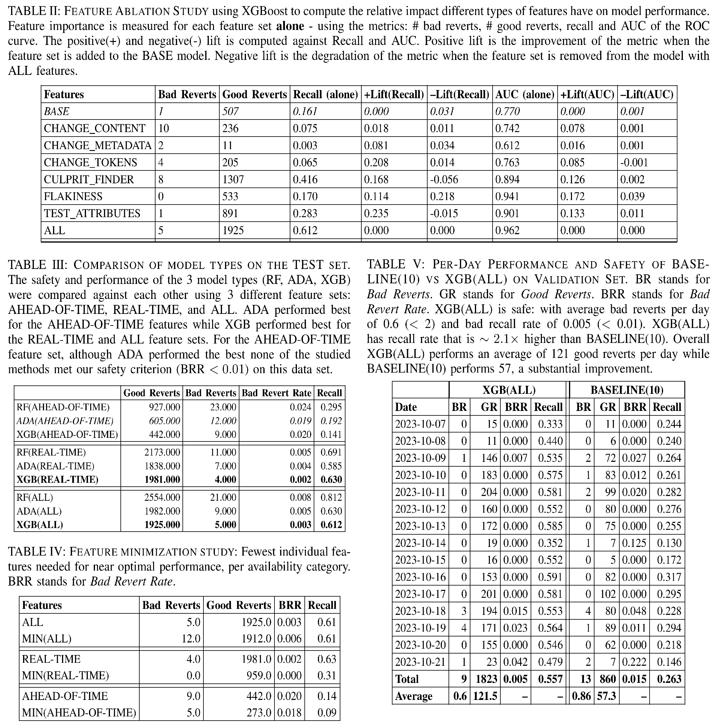
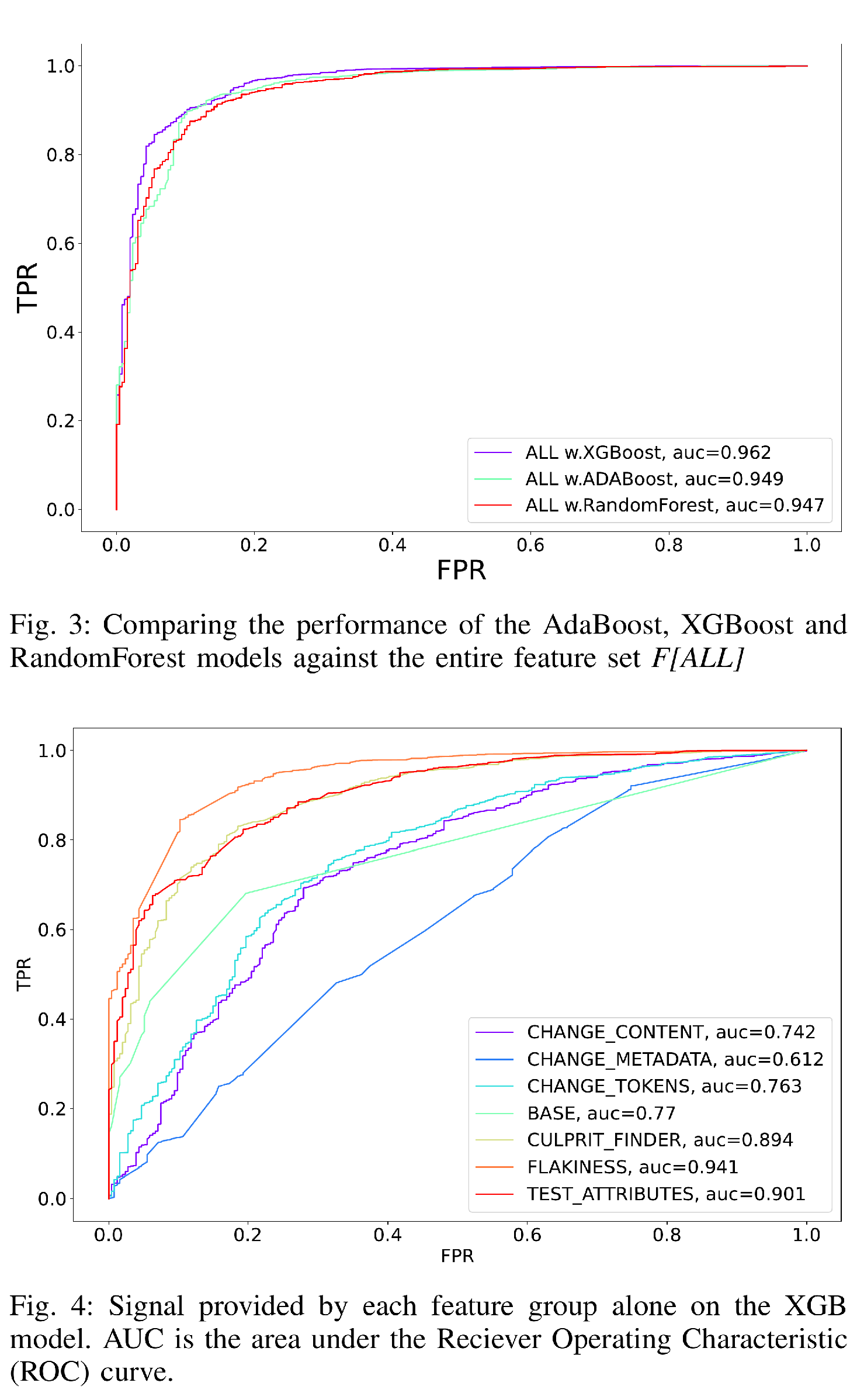
Table [table:model-comparison] summarizes the critical metrics for safety (bad revert rate) and performance (recall) for the three model types considered: RandomForest [RF], AdaBoost [ADA], and XGBoost [XGB]. Figure [fig:model-comparison] shows the Receiver Operator Curves (ROC) for all 3 model types and their associated area under the curve (AUC) values. The ROC curve better summarizes model performance over a wider range of target objectives than the table which is focused on the safest configuration (minimizing Bad Revert Rate). For instance if a different application had a higher tolerance for bad reversion/false positives the ROC curves show that you could achieve a 90% true positive rate with a 20% false positive rate.
Safety: In general, XGB and ADA both outperformed the RF in terms of safety. Under none of the test configurations did the RF have a safe configuration. XGB and ADA are safe (under our criteria, see Section 4.2) using all the features or the REAL-TIME subset. The safest configuration was XGB(ALL) which had only 5 bad reverts and a bad revert rate of 0.003. XGB(REAL-TIME) and ADA(ALL) has the same or smaller number of bad reverts but a worse rate due to their lower recall.
Performance: The highest performing configuration was XGB(ALL) which had 1980 Good Reverts in the Test set and a recall of 63.2%. The recall rate of XGB(REAL-TIME) was 52.2% indicating that most of the model performance is gained from the REAL-TIME features, not from the AHEAD-OF-TIME features which performed much worse while being unsafe. ADA(ALL) was safe but its recall rate was only 42.2% which lower than both safe XGB configurations.
RQ2: What is the marginal benefit provided by each feature group?
Summary: Historical flakiness data was the most valuable feature set, boosting model recall by 17%, while change metadata was the least important.
Note: This experiment was conducted on the TEST data set as the VALIDATION set was reserved for RQ3.
To determine marginal benefit we perform an ablation study to look at the marginal benefit provided by each feature (as grouped in Table 1). The ablation study was performed using the XGBoost model which was chosen over AdaBoost due to its higher recall as seen in Table [table:model-comparison]. Three marginal benefit experiments were performed:
Measure the performance of the model trained against only the features in a single feature set. We visualize the results in Figure [fig:feature-group-contrib] as an ROC curve. Table [table:feature-ablation] contains the critical safety and performance metrics of Bad Reverts (safety) and Recall (performance) as well as the AUC which summarizes overall model predictive performance – generally a model with a higher AUC will be more performant than one with a lower AUC.
Measure the Positive(+) Lift provided by adding a single feature group to our BASE feature (the number of blaming tests). For instance, we would add the features in CHANGE_CONTENT to create a XGB(CHANGE_CONTENT + BASE) model. The +Lift for Recall is computed as Recall[XGB(CHANGE_CONTENT + BASE)] - Recall[XGB(BASE)] and similar for AUC of the ROC curve. The results of this analysis are shown in Table [table:feature-ablation].
Measure the Negative(–) Lift provided by removing a single feature group from out ALL feature set. For instance we would remove the features in CHANGE_CONTENT to create a XGB(ALL - CHANGE_CONTENT) model. The –Lift for Recall is computed as Recall[XGB(ALL)] - Recall[XGB(ALL - CHANGE_CONTENT)] and similar for AUC of the ROC curve. The results of this analysis are shown in Table [table:feature-ablation].
As discussed in section 3.4.3, we attempted to minimize the feature subsets while providing comparable performance to the full feature sets. Table [table:featureMinimization] contains a breakdown of the performance for these minimal subsets.
RQ3:Did the chosen method improve performance over the baseline method while maintaining required safety levels?
Summary: XGB(ALL) improved overall recall while meeting our safety requirements with a Bad Revert Rate under 1% and an average of 0.6 Bad Reverts per Day. BASELINE(10) had a recall of 26.3% while XGB(ALL) had a recall of 55.7% – an improvement of \(\sim 2.1\times\).
Note: We used the reserved VALIDATION data set for this research question.
Table [table:validation-evaluation] shows per day metrics comparing XGB(ALL) against the heuristic BASELINE(10) method. XGB(ALL) was selected as our “OPTIMAL” model to compare against the BASELINE method given its performance in the TEST set as evaluated in RQ1. As a reminder the BASELINE method thresholds the number of blaming tests to a fixed number. BASELINE(10)’s average bad reverts per day is 0.86 and its total Bad Revert Rate (BRR) is 1.5%. XGB(ALL) achieves the overall safety limit with a BRR of 0.5% and has an average bad reverts per day of 0.6 which meets our safety threshold.
XGB(ALL)’s bad revert rate outperforms BASELINE(10), with a recall 2.1 times higher than BASELINE(10). XGB(ALL) made 1,823 total good reverts in the validation set while BASELINE(10) performed 860 good reverts. Based on the data in Table [table:validation-evaluation] XGB(ALL) is both safer and more performant than BASELINE(10) on the validation data set.
Discussion
The proposed method, SafeRevert, is generic and can be used with any culprit finding algorithm. By grouping individual features from different sources of data into logical feature sets (Table 1), performing a detailed feature ablation study (Fig [fig:feature-group-contrib]), and running the model on a minimal set of features (Table [table:featureMinimization]), we hope to provide a template via which teams in other contexts build on when adopting the approach we outline. In particular, while some features used may be Google specific, our feature ablation study can be replicated on different features in other software development organizations. While we don’t expect a team implementing SafeRevert to achieve the exact Recall and Bad Revert Rates we report we do expect this method to out perform the BASELINE method once an appropriate set of features is identified.
Threats to Validity
Our dataset may misrepresent information available at inference time in the forthcoming service as it may include information not available to us at our decision time. This is due to using offline data in the dataset as the production system based on this paper is currently under construction. We adjust this threat by evaluating performance restricted to features available independent of any culprit finding event and restricting our real-time data to a time bound relative to change submission time.
The data presented in this final manuscript differs slightly than the
reviewed manuscript. At the time of review approximated 15% of the
dataset was lacking verification results (collected using the method
described by Henderson (Henderson et al. 2023)). This was
disclosed in this section to the reviewers and we made two conservative
assumptions: 1) any culprit change lacking verification results was
considered a false positive and 2) we assumed the BASELINE method was
correct for those changes (inflating the BASELINE methods performance
versus the studied ML methods for SafeRevert). Since the peer review was
completed, a bug in the verification system was identified and fixed.
The bug caused a proportion of incorrect culprit changes to “get stuck”
in a queue waiting for an additional test execution due to a typo in a
comparison (using > instead of >=). Once
the bug was fixed, the research team was able to rerun the study with
the additional label data.
Post-rerun we observed: 1) the BASELINE method performed worse and 2) the studied methods were robust to the change in labeling data. In the reviewed manuscript, XGB(ALL) had the following results in RQ3: 13 Total Bad Reverts, 1817 Good Reverts, 0.7% Bad Revert Rate, and 55.8% Recall; BASELINE(5) was compared against and had 8 Total Bad Reverts, 1286 Good Reverts, 0.6% Bad Revert Rate, and 39.4% Recall. Compare against Table [table:validation-evaluation] and Figure [fig:baseline]. We switched to using BASELINE(10) for this final manuscript as it is the production method currently used at Google.
Related Work
In this paper, we are presenting what we believe to be a novel problem to the wider software engineering community: how to safely choose changes to revert with incomplete but suggestive evidence. This problem relies on identifying these problematic changes. In our case we identify the problematic changes to revert via automated culprit finding (Couder 2008; Ziftci and Ramavajjala 2013; Ziftci and Reardon 2017; Saha and Gligoric 2017; Najafi, Rigby, and Shang 2019; Beheshtian, Bavand, and Rigby 2022; Keenan 2019; An and Yoo 2021; Ocariza 2022; Henderson et al. 2023).
Culprit finding’s development has often occurred outside of the
academic literature. The first reference to the process of using binary
search to identify a bug was in Yourdon’s 1975 book on Program Design:
Page 286, Figure 8.3 titled “A binary search for bugs” (Yourdon 1975). The process is explained
in detail in the BUG-HUNTING file in the Linux source tree
in 1996 by Larry McVoy (McVoy 1996; Cox, Ness, and McVoy 2023). By 1997,
Brian Ness had created a binary search based system for use at Cray with
their “Unicos Source Manager” version control system (Ness and Ngo 1997; Cox, Ness, and McVoy 2023). Previously
in (Henderson et al.
2023) we had credited Linus Torvalds for the invention based
on lack of findable antecedent for his work on the
git bisect command (Couder 2008). We regret the error and
recognize the above individuals for their important contributions.
Other methods for identifying buggy code or breaking changes have been studied (some widely) in the literature. Fault Localization looks to identify the buggy code that is causing either operational failure or test failures (Agarwal and Agrawal 2014; Wong et al. 2016). Methods for fault localization include: delta debugging (Zeller 1999), statistical coverage based fault localization (J. a. Jones, Harrold, and Stasko 2002; J. A. Jones and Harrold 2005; Lucia et al. 2014; Henderson and Podgurski 2018; Henderson, Podgurski, and Kucuk 2019; Kucuk, Henderson, and Podgurski 2021), information retrieval (which may include historical information) (J. Zhou, Zhang, and Lo 2012; Youm et al. 2015; Ciborowska and Damevski 2022), and program slicing (Podgurski and Clarke 1990; Horwitz and Reps 1992; Ren et al. 2004).
Bug Prediction attempts to predict if a change, method, class, or file is likely to contain a bug (Lewis et al. 2013; Punitha and Chitra 2013; Osman et al. 2017). This idea has conceptual similarities to the work we are doing in this paper where we are using similar metrics to predict whether or not a change which has been implicated by culprit finding is in fact the change that introduced the bug. Our methods could be potentially improved by incorporating the additional features used in the bug prediction work such as the change complexity, code complexity, and object-oriented complexity metrics.
Test Case Selection (Leon and Podgurski 2003; Engström, Runeson, and Skoglund 2010; Z. Q. Zhou 2010; Mondal, Hemmati, and Durocher 2015; Musa et al. 2015; Pan et al. 2022) and Test Case Prioritization (Singh et al. 2012; de S. Campos Junior et al. 2017; De Castro-Cabrera, García-Dominguez, and Medina-Bulo 2020; Pan et al. 2022) are related problems to the change reversion problem we study. Instead of predicting whether or not a change caused a known test failure in Test Case Selection/Prioritization often the change is used to predict whether a given test will fail before it is run. There is a large body work in that uses dynamic information from past test executions (such as code coverage) to inform the selection process. We believe this hints that such information could be highly informative for the change reversion problem as well.
Finally, there are a family of methods for finding bug inducing commits for the purpose of supporting studies that data mine software repositories (Śliwerski, Zimmermann, and Zeller 2005; Rodríguez-Pérez, Robles, and González-Barahona 2018; Borg et al. 2019; Wen et al. 2019; An et al. 2023). These methods typically used to conduct a historical analysis of a repository rather than as an online detection as in culprit finding.
Conclusion
We presented: SafeRevert a method for improving systems that automatically revert changes that break tests. SafeRevert was developed as a way to improve the number bad changes automatically reverted while maintaining safety (rarely reverting good changes). To evaluate SafeRevert, we performed an empirical evaluation comparing the performance of SafeRevert against the baseline method that is currently utilized in production which utilizes a simple heuristic to determine if a change is safe to revert: the number of tests which “blame” the culprit change. When evaluating RQ3 in Section 5, it was observed that the XGB(ALL) configuration of SafeRevert doubled the number changes reverted while reducing the number of bad reverts performed (see Table [table:validation-evaluation]).
While it is unlikely that a replication study in a different development environment would reproduce our exact results we do expect based on the robust difference observed between SafeRevert and BASELINE that SafeRevert (or similar ML based method) will be able to improve the number of changes eligible for automatic reversion. We hope that by introducing this problem to the larger software engineering community that new and innovative approaches to solving it will be developed.
References
- Agarwal, Pragya, and Arun Prakash Agrawal. 2014. “Fault-Localization Techniques for Software Systems: A Literature Review.” SIGSOFT Softw. Eng. Notes 39 (5): 1–8. https://doi.org/10.1145/2659118.2659125.
- An, Gabin, Jingun Hong, Naryeong Kim, and Shin Yoo. 2023. “Fonte: Finding Bug Inducing Commits from Failures.” arXiv. http://arxiv.org/abs/2212.06376.
- An, Gabin, and Shin Yoo. 2021. “Reducing the Search Space of Bug Inducing Commits Using Failure Coverage.” In Proceedings of the 29th ACM Joint Meeting on European Software Engineering Conference and Symposium on the Foundations of Software Engineering, 1459–62. Athens Greece: ACM. https://doi.org/10.1145/3468264.3473129.
- Ananthanarayanan, Sundaram, Masoud Saeida Ardekani, Denis Haenikel, Balaji Varadarajan, Simon Soriano, Dhaval Patel, and Ali Reza Adl-Tabatabai. 2019. “Keeping Master Green at Scale.” Proceedings of the 14th EuroSys Conference 2019. https://doi.org/10.1145/3302424.3303970.
- Beheshtian, Mohammad Javad, Amir Hossein Bavand, and Peter C. Rigby. 2022. “Software Batch Testing to Save Build Test Resources and to Reduce Feedback Time.” IEEE Transactions on Software Engineering 48 (8): 2784–2801. https://doi.org/10.1109/TSE.2021.3070269.
- Ben-Or, Michael, and Avinatan Hassidim. 2008. “The Bayesian Learner Is Optimal for Noisy Binary Search (and Pretty Good for Quantum as Well).” In 2008 49th Annual IEEE Symposium on Foundations of Computer Science, 221–30. Philadelphia, PA, USA: IEEE. https://doi.org/10.1109/FOCS.2008.58.
- Bland, Mike. 2012. “The Chris/Jay Continuous Build.” Personal {{Website}}. Mike Bland’s Blog. https://mike-bland.com/2012/06/21/chris-jay-continuous- build.html.
- Borg, Markus, Oscar Svensson, Kristian Berg, and Daniel Hansson. 2019. “SZZ Unleashed: An Open Implementation of the SZZ Algorithm - Featuring Example Usage in a Study of Just-in-Time Bug Prediction for the Jenkins Project.” In Proceedings of the 3rd ACM SIGSOFT International Workshop on Machine Learning Techniques for Software Quality Evaluation - MaLTeSQuE 2019, 7–12. Tallinn, Estonia: ACM Press. https://doi.org/10.1145/3340482.3342742.
- Chen, Tianqi, and Carlos Guestrin. 2016. “XGBoost: A Scalable Tree Boosting System.” In Proceedings of the 22nd ACM SIGKDD International Conference on Knowledge Discovery and Data Mining, 785–94. San Francisco California USA: ACM. https://doi.org/10.1145/2939672.2939785.
- Ciborowska, Agnieszka, and Kostadin Damevski. 2022. “Fast Changeset-Based Bug Localization with BERT.” In Proceedings of the 44th International Conference on Software Engineering, 946–57. Pittsburgh Pennsylvania: ACM. https://doi.org/10.1145/3510003.3510042.
- Couder, Christian. 2008. “Fighting Regressions with Git Bisect.” The Linux Kernel Archives 4 (5). https://www. kernel. org/pub/software/scm/git/doc s/git- bisect-lk2009.html.
- Cox, Russ, Brian Ness, and Larry McVoy. 2023. “Comp.lang.compilers "Binary Search Debugging of Compilers".” https://groups.google.com/g/comp.compilers/c/vGh4s3HBQ-s/m/ Chvpu7vTAgAJ.
- De Castro-Cabrera, M. Del Carmen, Antonio García-Dominguez, and Inmaculada Medina-Bulo. 2020. “Trends in Prioritization of Test Cases: 2017-2019.” Proceedings of the ACM Symposium on Applied Computing, 2005–11. https://doi.org/10.1145/3341105.3374036.
- de S. Campos Junior, Heleno, Marco Antônio P Araújo, José Maria N David, Regina Braga, Fernanda Campos, and Victor Ströele. 2017. “Test Case Prioritization: A Systematic Review and Mapping of the Literature.” In Proceedings of the 31st Brazilian Symposium on Software Engineering, 34–43. New York, NY, USA: ACM. https://doi.org/10.1145/3131151.3131170.
- Engström, Emelie, Per Runeson, and Mats Skoglund. 2010. “A Systematic Review on Regression Test Selection Techniques.” Information and Software Technology 52 (1): 14–30. https://doi.org/10.1016/j.infsof.2009.07.001.
- Fowler, Martin. 2006. “Continuous Integration.” https://martinfowler.com/articles/ continuousIntegration.html.
- Gupta, Pooja, Mark Ivey, and John Penix. 2011. “Testing at the Speed and Scale of Google.” http://google-engtools.blogspot.com/2011/06/testing-at- speed-and-scale-of-google.html.
- Henderson, Tim A. D., Bobby Dorward, Eric Nickell, Collin Johnston, and Avi Kondareddy. 2023. “Flake Aware Culprit Finding.” In 2023 IEEE Conference on Software Testing, Verification and Validation (ICST). IEEE. https://hackthology.com/flake-aware-culprit-finding.html. https://doi.org/10.1109/ICST57152.2023.00041.
- Henderson, Tim A. D., and Andy Podgurski. 2018. “Behavioral Fault Localization by Sampling Suspicious Dynamic Control Flow Subgraphs.” In 2018 IEEE 11th International Conference on Software Testing, Verification and Validation (ICST), 93–104. Vasteras: IEEE. https://hackthology.com/behavioral-fault-localization-by-sampling-suspicious-dynamic-control-flow-subgraphs.html. https://doi.org/10.1109/ICST.2018.00019.
- Henderson, Tim A. D., Andy Podgurski, and Yigit Kucuk. 2019. “Evaluating Automatic Fault Localization Using Markov Processes.” In 2019 19th International Working Conference on Source Code Analysis and Manipulation (SCAM), 115–26. Cleveland, OH, USA: IEEE. https://hackthology.com/evaluating-automatic-fault-localization-using-markov-processes.html https://doi.org/10.1109/SCAM.2019.00021.
- Herzig, Kim, and Nachiappan Nagappan. 2015. “Empirically Detecting False Test Alarms Using Association Rules.” In 2015 IEEE/ACM 37th IEEE International Conference on Software Engineering, 39–48. Florence, Italy: IEEE. https://doi.org/10.1109/ICSE.2015.133.
- Horwitz, S, and T Reps. 1992. “The Use of Program Dependence Graphs in Software Engineering.” In International Conference on Software Engineering, 9:349. Springer. http://portal.acm.org/citation.cfm?id=24041&dl=.
- Jones, J.a., M. J. Harrold, and J. Stasko. 2002. “Visualization of Test Information to Assist Fault Localization.” Proceedings of the 24th International Conference on Software Engineering. ICSE 2002. https://doi.org/10.1145/581339.581397.
- Jones, James A., and Mary Jean Harrold. 2005. “Empirical Evaluation of the Tarantula Automatic Fault-localization Technique.” In Proceedings of the 20th IEEE/ACM International Conference on Automated Software Engineering, 273–82. New York, NY, USA: ACM. https://doi.org/10.1145/1101908.1101949.
- Keenan, James. 2019. “James E. Keenan - "Multisection: When Bisection Isn’t Enough to Debug a Problem".” https://www.youtube.com/watch?v=05CwdTRt6AM.
- Kucuk, Yigit, Tim A. D. Henderson, and Andy Podgurski. 2021. “Improving Fault Localization by Integrating Value and Predicate Based Causal Inference Techniques.” In 2021 IEEE/ACM 43rd International Conference on Software Engineering (ICSE), 649–60. Madrid, ES: IEEE. https://doi.org/10.1109/ICSE43902.2021.00066.
- Leon, D., and A. Podgurski. 2003. “A Comparison of Coverage-Based and Distribution-Based Techniques for Filtering and Prioritizing Test Cases.” In 14th International Symposium on Software Reliability Engineering, 2003. ISSRE 2003., 2003-Janua:442–53. IEEE. https://doi.org/10.1109/ISSRE.2003.1251065.
- Leong, Claire, Abhayendra Singh, Mike Papadakis, Yves Le Traon, and John Micco. 2019. “Assessing Transition-Based Test Selection Algorithms at Google.” In 2019 IEEE/ACM 41st International Conference on Software Engineering: Software Engineering in Practice (ICSE-SEIP), 101–10. IEEE. https://doi.org/10.1109/ICSE-SEIP.2019.00019.
- Lewis, Chris, Zhongpeng Lin, Caitlin Sadowski, and Xiaoyan Zhu. 2013. “Does Bug Prediction Support Human Developers? Findings from a Google Case Study.” In Proceedings of the …, 372–81. http://dl.acm.org/citation.cfm?id=2486838.
- Lucia, David Lo, Lingxiao Jiang, Ferdian Thung, and Aditya Budi. 2014. “Extended Comprehensive Study of Association Measures for Fault Localization.” Journal of Software: Evolution and Process 26 (2): 172–219. https://doi.org/10.1002/smr.1616.
- Machalica, Mateusz, Alex Samylkin, Meredith Porth, and Satish Chandra. 2019. “Predictive Test Selection.” In 2019 IEEE/ACM 41st International Conference on Software Engineering: Software Engineering in Practice (ICSE-SEIP), 91–100. IEEE. https://doi.org/10.1109/ICSE-SEIP.2019.00018.
- McVoy, Larry. 1996. “BUG-HUNTING.” linux/1.3.73. https://elixir.bootlin.com/linux/1.3.73/source/ Documentation/BUG-HUNTING.
- Memon, Atif, Zebao Gao, Bao Nguyen, Sanjeev Dhanda, Eric Nickell, Rob Siemborski, and John Micco. 2017. “Taming Google-scale Continuous Testing.” In 2017 IEEE/ACM 39th International Conference on Software Engineering: Software Engineering in Practice Track (ICSE-SEIP), 233–42. Piscataway, NJ, USA: IEEE. https://doi.org/10.1109/ICSE-SEIP.2017.16.
- Micco, John. 2012. “Tools for Continuous Integration at Google Scale.” Tech {{Talk}}. Google NYC. https://youtu.be/KH2_sB1A6lA.
- ———. 2013. “Continuous Integration at Google Scale.” Lecture. EclipseCon 2013. https://web.archive.org/web/20140705215747/https:// www.eclipsecon.org/2013/sites/eclipsecon.org.2013/files/2013- 03-24%20Continuous%20Integration%20at%20Google%20Scale.pdf.
- Mondal, Debajyoti, Hadi Hemmati, and Stephane Durocher. 2015. “Exploring Test Suite Diversification and Code Coverage in Multi-Objective Test Case Selection.” 2015 IEEE 8th International Conference on Software Testing, Verification and Validation, ICST 2015 - Proceedings, 1–10. https://doi.org/10.1109/ICST.2015.7102588.
- Musa, Samaila, Abu Bakar Md Sultan, Abdul Azim Bin Abd-Ghani, and Salmi Baharom. 2015. “Regression Test Cases Selection for Object-Oriented Programs Based on Affected Statements.” International Journal of Software Engineering and Its Applications 9 (10): 91–108. https://doi.org/10.14257/ijseia.2015.9.10.10.
- Najafi, Armin, Peter C. Rigby, and Weiyi Shang. 2019. “Bisecting Commits and Modeling Commit Risk During Testing.” In Proceedings of the 2019 27th ACM Joint Meeting on European Software Engineering Conference and Symposium on the Foundations of Software Engineering, 279–89. New York, NY, USA: ACM. https://doi.org/10.1145/3338906.3338944.
- Najafi, Armin, Weiyi Shang, and Peter C. Rigby. 2019. “Improving Test Effectiveness Using Test Executions History: An Industrial Experience Report.” In 2019 IEEE/ACM 41st International Conference on Software Engineering: Software Engineering in Practice (ICSE-SEIP), 213–22. IEEE. https://doi.org/10.1109/ICSE-SEIP.2019.00031.
- Ness, B., and V. Ngo. 1997. “Regression Containment Through Source Change Isolation.” In Proceedings Twenty-First Annual International Computer Software and Applications Conference (COMPSAC’97), 616–21. Washington, DC, USA: IEEE Comput. Soc. https://doi.org/10.1109/CMPSAC.1997.625082.
- Ocariza, Frolin S. 2022. “On the Effectiveness of Bisection in Performance Regression Localization.” Empirical Software Engineering 27 (4): 95. https://doi.org/10.1007/s10664-022-10152-3.
- Osman, Haidar, Mohammad Ghafari, Oscar Nierstrasz, and Mircea Lungu. 2017. “An Extensive Analysis of Efficient Bug Prediction Configurations.” In Proceedings of the 13th International Conference on Predictive Models and Data Analytics in Software Engineering, 107–16. Toronto Canada: ACM. https://doi.org/10.1145/3127005.3127017.
- Pan, Rongqi, Mojtaba Bagherzadeh, Taher A. Ghaleb, and Lionel Briand. 2022. “Test Case Selection and Prioritization Using Machine Learning: A Systematic Literature Review.” Empirical Software Engineering 27 (2): 29. https://doi.org/10.1007/s10664-021-10066-6.
- Parry, Owain, Gregory M. Kapfhammer, Michael Hilton, and Phil McMinn. 2022. “A Survey of Flaky Tests.” ACM Transactions on Software Engineering and Methodology 31 (1): 1–74. https://doi.org/10.1145/3476105.
- Pedregosa, F., G. Varoquaux, A. Gramfort, V. Michel, B. Thirion, O. Grisel, M. Blondel, et al. 2011. “Scikit-Learn: Machine Learning in Python.” Journal of Machine Learning Research 12: 2825–30.
- Pelc, Andrzej. 2002. “Searching Games with Errorsfifty Years of Coping with Liars.” Theoretical Computer Science 270 (1-2): 71–109. https://doi.org/10.1016/S0304-3975(01)00303-6.
- Podgurski, A, and L A Clarke. 1990. “A Formal Model of Program Dependences and Its Implications for Software Testing, Debugging, and Maintenance.” IEEE Transactions of Software Engineering 16 (9): 965–79. https://doi.org/10.1109/32.58784.
- Potvin, Rachel, and Josh Levenberg. 2016. “Why Google Stores Billions of Lines of Code in a Single Repository.” Communications of the ACM 59 (7): 78–87. https://doi.org/10.1145/2854146.
- Punitha, K., and S. Chitra. 2013. “Software Defect Prediction Using Software Metrics - A Survey.” In 2013 International Conference on Information Communication and Embedded Systems (ICICES), 555–58. Chennai: IEEE. https://doi.org/10.1109/ICICES.2013.6508369.
- Ren, Xiaoxia, Fenil Shah, Frank Tip, Barbara G. Ryder, and Ophelia Chesley. 2004. “Chianti: A Tool for Change Impact Analysis of Java Programs.” In Proceedings of the 19th Annual ACM SIGPLAN Conference on Object-oriented Programming, Systems, Languages, and Applications, 432–48. Vancouver BC Canada: ACM. https://doi.org/10.1145/1028976.1029012.
- Rivest, R. L., A. R. Meyer, and D. J. Kleitman. 1978. “Coping with Errors in Binary Search Procedures (Preliminary Report).” In Proceedings of the Tenth Annual ACM Symposium on Theory of Computing - STOC ’78, 227–32. San Diego, California, United States: ACM Press. https://doi.org/10.1145/800133.804351.
- Rodríguez-Pérez, Gema, Gregorio Robles, and Jesús M. González-Barahona. 2018. “Reproducibility and Credibility in Empirical Software Engineering: A Case Study Based on a Systematic Literature Review of the Use of the SZZ Algorithm.” Information and Software Technology 99 (July): 164–76. https://doi.org/10.1016/j.infsof.2018.03.009.
- Saha, Ripon, and Milos Gligoric. 2017. “Selective Bisection Debugging.” In Fundamental Approaches to Software Engineering, edited by Marieke Huisman and Julia Rubin, 10202:60–77. Berlin, Heidelberg: Springer Berlin Heidelberg. https://doi.org/10.1007/978-3-662-54494-5_4.
- Singh, Yogesh, Arvinder Kaur, Bharti Suri, and Shweta Singhal. 2012. “Systematic Literature Review on Regression Test Prioritization Techniques.” Informatica (Slovenia) 36 (4): 379–408. https://doi.org/10.31449/inf.v36i4.420.
- Śliwerski, Jacek, Thomas Zimmermann, and Andreas Zeller. 2005. “When Do Changes Induce Fixes?” ACM SIGSOFT Software Engineering Notes 30 (4): 1. https://doi.org/10.1145/1082983.1083147.
- Wang, Kaiyuan, Greg Tener, Vijay Gullapalli, Xin Huang, Ahmed Gad, and Daniel Rall. 2020. “Scalable Build Service System with Smart Scheduling Service.” In Proceedings of the 29th ACM SIGSOFT International Symposium on Software Testing and Analysis, 452–62. Virtual Event USA: ACM. https://doi.org/10.1145/3395363.3397371.
- Wen, Ming, Rongxin Wu, Yepang Liu, Yongqiang Tian, Xuan Xie, Shing-Chi Cheung, and Zhendong Su. 2019. “Exploring and Exploiting the Correlations Between Bug-Inducing and Bug-Fixing Commits.” In Proceedings of the 2019 27th ACM Joint Meeting on European Software Engineering Conference and Symposium on the Foundations of Software Engineering, 326–37. Tallinn Estonia: ACM. https://doi.org/10.1145/3338906.3338962.
- Wong, W. Eric, Ruizhi Gao, Yihao Li, Rui Abreu, and Franz Wotawa. 2016. “A Survey on Software Fault Localization.” IEEE Transactions on Software Engineering 42 (8): 707–40. https://doi.org/10.1109/TSE.2016.2521368.
- Youm, Klaus Changsun, June Ahn, Jeongho Kim, and Eunseok Lee. 2015. “Bug Localization Based on Code Change Histories and Bug Reports.” In 2015 Asia-Pacific Software Engineering Conference (APSEC), 190–97. New Delhi: IEEE. https://doi.org/10.1109/APSEC.2015.23.
- Yourdon, E. 1975. Techniques of Program Design. New Jersey: Prentice-Hall.
- Zeller, Andreas. 1999. “Yesterday, My Program Worked. Today, It Does Not. Why?” SIGSOFT Softw. Eng. Notes 24 (6): 253–67. https://doi.org/10.1145/318774.318946.
- Zhou, Jian, Hongyu Zhang, and David Lo. 2012. “Where Should the Bugs Be Fixed? More Accurate Information Retrieval-Based Bug Localization Based on Bug Reports.” Proceedings - International Conference on Software Engineering, 14–24. https://doi.org/10.1109/ICSE.2012.6227210.
- Zhou, Zhi Quan. 2010. “Using Coverage Information to Guide Test Case Selection in Adaptive Random Testing.” Proceedings - International Computer Software and Applications Conference, 208–13. https://doi.org/10.1109/COMPSACW.2010.43.
- Ziftci, Celal, and Vivek Ramavajjala. 2013. “Finding Culprits Automatically in Failing Builds - i.e. Who Broke the Build?” https://www.youtube.com/watch?v=SZLuBYlq3OM.
- Ziftci, Celal, and Jim Reardon. 2017. “Who Broke the Build? Automatically Identifying Changes That Induce Test Failures in Continuous Integration at Google Scale.” Proceedings - 2017 IEEE/ACM 39th International Conference on Software Engineering: Software Engineering in Practice Track, ICSE-SEIP 2017, 113–22. https://doi.org/10.1109/ICSE-SEIP.2017.13.
Both the per-test error rate and the per-change error rates quoted above are drawn from the same 28 day window. The Postsubmit result which triggers culprit finding may itself have been a flake, so there were spurious suspect ranges in the same period. These rates may differ slightly from the numbers reported in (Henderson et al. 2023) as they reflect our most recent data as of 2023-11-12.↩︎
There are some legacy tests which are allowed to use the network but there is an on-going effort to clean up their usage.↩︎
Previously, we referred to these cycles as “Milestones” in most of the previous literature but we are gradually changing our internal nomenclature as we evolve TAP Postsubmit’s testing model.↩︎
https://scikit-learn.org/↩︎