Evaluating Automatic Fault Localization Using Markov Processes
Tim A. D. Henderson, Yiğit Küçük, and Andy Podgurski
Evaluating Automatic Fault Localization Using Markov Processes. SCAM 2019.
DOI.
PDF.
SUPPLEMENT.
WEB.
Note
This is a conversion from a latex paper I wrote. If you want all formatting correct you should read the pdf version.
Abstract
Statistical fault localization (SFL) techniques are commonly compared and evaluated using a measure known as "Rank Score" and its associated evaluation process. In the latter process each SFL technique under comparison is used to produce a list of program locations, ranked by their suspiciousness scores. Each technique then receives a Rank Score for each faulty program it is applied to, which is equal to the rank of the first faulty location in the corresponding list. The SFL technique whose average Rank Score is lowest is judged the best overall, based on the assumption that a programmer will examine each location in rank order until a fault is found. However, this assumption *oversimplifies* how an SFL technique would be used in practice. Programmers are likely to regard suspiciousness ranks as just one source of information among several that are relevant to locating faults. This paper provides a new evaluation approach using first-order Markov models of debugging processes, which can incorporate multiple additional kinds of information, e.g., about code locality, dependences, or even intuition. Our approach, \( \textrm{HT}_{\textrm{Rank}} \), scores SFL techniques based on the expected number of steps a programmer would take through the Markov model before reaching a faulty location. Unlike previous evaluation methods, \(\textrm{HT}_{\textrm{Rank}}\) can compare techniques even when they produce fault localization reports differing in structure or information granularity. To illustrate the approach, we present a case study comparing two existing fault localization techniques that produce results varying in form and granularity.
Introduction
Automatic fault localization is a software engineering technique to assist a programmer during the debugging process by suggesting "suspicious" locations that may contain or overlap with a fault (bug, defect) that is the root cause of observed failures. The big idea behind automatic fault localization (or just fault localization) is that pointing the programmer towards the right area of the program will enable them to find the relevant fault more quickly.
A much-investigated approach to fault localization is Coverage-Based Statistical Fault Localization (CBSFL), which is also known as Spectrum-Based Fault Localization [1]-[3]. This approach uses code-coverage profiles and success/failure information from testing or field use of software to rank statements or other generic program locations (e.g., basic blocks, methods, or classes) from most "suspicious" (likely to be faulty) to least suspicious. To perform CBSFL, each test case is run using a version of the program being debugged that has been instrumented to record which potential fault locations were actually executed on that test. A human or automated test oracle labels each test to indicate whether it passed or failed. The coverage profiles are also referred to as coverage spectra.
In the usage scenario typically envisioned for CBSFL, a programmer uses the ranked list of program locations to guide debugging. Starting at the top of the list and moving down, they examine each location to determine if it is faulty. If the location of a fault is near the top of the list, the programmer saves time by avoiding consideration of most of the non-faulty locations in the program. However, if there is no fault near the top of the list, the programmer instead wastes time examining many more locations than necessary. CBSFL techniques are typically evaluated empirically in terms of their ability to rank faulty locations near the top of the list [4], [5], as measured by each technique's "Rank Score", which is the location of the first faulty location in the list. A CBSFL technique that consistently ranks faulty statements from a wide range of faulty programs near the top of the corresponding lists is considered a good technique.
One pitfall of using the ranked-list evaluation regime outlined above is that it can be applied fairly only when the techniques being compared provide results as a prioritized list of program elements of the same granularity. This means that if technique A produces a prioritized list of basic blocks, technique B produces an unordered set of sub-expressions, and technique C produces a prioritized list of classes then it is not valid to use the Standard Rank Score to compare them. The Standard Rank Score can only be applied to ordered lists and thus cannot be used directly to evaluate technique B, and it requires the techniques being compared to have the same granularity. Our new evaluation metric (called \(\textrm{HT}_{\textrm{Rank}}\)) accounts for these differences in granularity and report construction, allowing a direct comparison between different styles of fault localization. We present a case study in Section 27 comparing behavioral fault localization (which produces fragments of the dynamic control flow graph) to standard CBSFL.
Second, it is evident that the imagined usage scenario for CBSFL, in which a programmer examines each possible fault location in rank order until a fault is found, is an oversimplification of programmer behavior [6]. Programmers are likely to deviate from this scenario, e.g.: by choosing not to re-examine locations that have already been carefully examined and have not changed; by examining the locations around a highly ranked one, regardless of their ranks; by examining locations that a highly ranked location is dependent upon or that are dependent upon it [7]; by employing a conventional debugger (such as gdb, WinDB, or Visual Studio's debugger); or simply by using their knowledge and intuition about the program.
To support more flexible and nuanced evaluation criteria for CBSFL and other fault localization techniques, we present a new approach to evaluating them that is based on constructing and analyzing first-order Markov models of debugging processes and that uses a new evaluation metric (\(\textrm{HT}_{\textrm{Rank}}\)) based on the "hitting time" of a Markov process. This approach allows researchers to directly compare different fault localization techniques by incorporating their results and other relevant information into an appropriate model. To illustrate the approach, we present models for two classes of fault localization techniques: CBSFL and Suspicious Behavior Based Fault Localization (SBBFL) [8], [9]. The models we present are also easy to update, allowing researchers to incorporate results of future studies of programmers' behavior during debugging.
Our new debugging model (and its \(\textrm{HT}_{\textrm{Rank}}\) metric) can be thought of as a first-order simulation of the debugging process as conducted by a programmer. As such, we intend for it to be a practical alternative to conducting an expensive user study. The model is capable of incorporating a variety of behaviors a programmer may exhibit while debugging, allowing researchers to evaluate the performance of their tool against multiple debugging "styles."
Background and Related Work
Coverage Based Statistical Fault Localization (CBSFL) [1], [4] techniques attempt to quantify the likelihood that individual program locations are faulty using sample statistics, called suspiciousness metrics or fault localization metrics, which are computed from PASS/FAIL labels assigned to test executions and from coverage profiles (coverage spectra) collected from those executions. A CBSFL suspiciousness metric (of which there are a great many [2], [3]) measures the statistical association between the occurrence of test failures and the coverage of individual program locations (program elements) of a certain kind.
Some statistical fault localization techniques use additional information beyond basic coverage information to either improve accuracy or provide more explainable results. For instance, work on Causal Statistical Fault Localization uses information about the execution of program dependence predecessors of a target statement to adjust for confounding bias that can distort suspiciousness scores [10]. By contrast, Suspicious-Behavior-Based Fault Localization (SBBFL) techniques use runtime control-flow information (the behavior) to identify groups of "collaborating" suspicious elements [9]. These techniques typically leverage data mining techniques [11] such as frequent pattern mining [12]-[14] or significant pattern mining [9], [15]. Unlike CBSFL techniques, SBBFL techniques output a ranked list of patterns (subgraphs, itemsets, trees) which each contain multiple program locations. This makes it difficult to directly compare SBBFL and CBSFL techniques using traditional evaluation methods.
Finally, a variety of non-statistical (or hybrid) approaches to fault localization have been explored [16]-[19]. These approaches range from delta debugging [20] to nearest neighbor queries [7] to program slicing [21], [22] to information retrieval [23]-[25] to test case generation [26]-[28]. Despite technical and theoretical differences in these approaches, they all suggest locations (or groups of locations) for programmers to consider when debugging.
The Tarantula Evaluation
Some of the earliest papers on fault localization do not provide a quantitative method for evaluating performance (as is seen in later papers [5]). For instance, the earliest CBSFL paper [1], by Jones et al., proposes a technique and evaluates it qualitatively using data visualization. At the time, this was entirely appropriate as Jones was proposing a technique for visualizing the relative suspiciousness of different statements, as estimated with what is now called a suspiciousness metric (Tarantula). The visualization used for evaluating this technique aggregated the visualizations for all of the subject programs included in the study.
While the evaluation method used in the Jones et al. paper [1] effectively communicated the potential of CBSFL (and interested many researchers in the idea) it was not good way to compare multiple fault localization techniques. In 2005 Jones and Harrold [4] published a study that compared their Tarantula technique to three other techniques: Set Union and Intersection [29], Nearest Neighbor [7], and Cause-Transitions [30]. These techniques involved different approaches toward the fault localization problem and originally had been evaluated in different ways. Jones and Harrold re-evaluated all of the techniques under a new common evaluation framework.
In their 2005 paper, Jones and Harrold evaluated the effectiveness of each fault localization technique by using it to rank the statements in each subject program version from most likely to be the root cause of observed program failures to least likely. For their technique Tarantula, the statements were ranked using the Tarantula suspiciousness score.1 To compare the effectiveness of the techniques, another kind of score was assigned to each faulty version of each subject program. This score is based on the "rank score":
Definition. Tarantula Rank Score [4]
Given a set of locations \(L\) with their suspiciousness scores \(s(l)\) for \(l \in L\) the Rank Score \(r(l)\) for a faulty location \(l \in L\) is: \[\begin{aligned} {{\left|{ \left\{ x ~:~ x \in L \wedge s(x) \ge s(l) \right\} }\right|}} \end{aligned}\]
For Set Union and Intersection, Nearest Neighbor, and Cause-Transitions, Jones and Harrold used an idea of Renieres and Reiss [7] and ranked a program's statements based on consideration of its System Dependence Graph (SDG) [31]. The surrogate suspiciousness score of a program location \(L\) is the inverse of the size of the smallest dependence sphere around \(L\) that contains a faulty location. The surrogate scores are then used to calculate the Tarantula Rank Score (Def. 14).
In Jones's and Harrold's evaluation the authors did not use the Tarantula Rank Score directly but instead used a version of it that is normalized by program size:
Definition. Tarantula Effectiveness Score (Expense) [4]
This score is the proportion of program locations that do not need to be examined to find a fault when the locations are examined in rank order. Formally, let \(n\) be the total number of program locations, and let \(r(f)\) be the Tarantula Rank Score (Def. 14) of the faulty location \(f\). Then the score is: \[\begin{aligned} \frac{n-r(f)}{n} \end{aligned}\]
Using the normalized effectiveness score, Jones and Harrold directly compared the fault localization effectiveness of the techniques they considered. They did this in two ways. First, they presented a table that bucketed all the buggy versions of all the programs by their Tarantula Effectiveness Scores (given as percentages). Second, they presented a figure that showed the same data as a cumulative curve.
The core ideas of Jones' and Harrold's Effectivness/Expense score now underlie most evaluations of CBSFL techniques. Faulty statements are scored, ranked, rank-scored, normalized, and then aggregated over all programs and versions to provide an overall representation of a fault localization method's performance (e.g., [53], [2], [3], [32]-[34]). However, some refinements have been made to both the Rank Score and the Effectiveness Score.
The Implied Debugging Models
It is worth (re)stating here the debugging model implied in the Jones and Harrold evaluation [4]. The programmer receives from the fault localization tool a ranked list of statements with the most suspicious statements at the top. The programmer then moves down the list examining each location in turn. If multiple statements have the same rank (the same suspiciousness score) all of those statements are examined before the programmer makes a determination on whether or not the bug has been located. This rule is captured in the mathematical definition of the Tarantula Rank Score (Definition 14).
For the non-CBSFL methods which Jones compared CBSFL against, the ranks of the program locations were once again compared using the method of Renieres and Reiss [7], [30], [35] which is sometimes called T-Score. As a reminder, this method computes a surrogate suspiciousness score based on the size of smallest dependence sphere2 centered around the locations indicated in the fault localization report that contain the faulty code. This implies a debugging model in which the programmer examines each "shell" of the dependence sphere in turn before moving onto the next larger shell (see Figure 7 in [30] for a visualization).
Neither of these debugging models are realistic. Programmers may be reasonably expected to deviate from the ordering implied by the ranking. During the debugging process a programmer may use a variety of information sources — including intuition — to decide on the next element to examine. They may examine the same element multiple times. They may take a highly circuitous route to the buggy code or via intuition jump immediately to the fault. The models described above allow for none of these subtleties.
Refinements to the Evaluation Framework
Wong et al. [32] introduced the most commonly used effectiveness score, which is called the \(\mathcal{EXAM}\) score. This score is essentially the same as the Expense score (Def. 15) except that it gives the percentage of locations that need to be examined rather than those avoided.
Definition. \(\mathcal{EXAM}\) Score [32]
\[\begin{aligned} \frac{r(f)}{n} \end{aligned}\]
Ali et al. [37] identified an important problem with Jones' and Harrold's evaluation method: some fault localization techniques always assign different locations distinct suspiciousness scores, but others do not. Ali et al. pointed out that when comparing techniques, the Tarantula Effectiveness Score may favor a technique that generates more distinct suspiciousness scores than the other techniques. The fix they propose is to assign to a location in a group of locations with the same suspiciousness score a rank score that reflects developers having to examine half the locations in the group on average.
Definition. Standard Rank Score
This score is the expected number of locations a programmer would inspect before locating a fault. Formally, given a set of locations \(L\) with their suspiciousness scores \(s(l)\) for \(l \in L\), the Rank Score for a location \(l \in L\) is [37]: \[\begin{aligned} {{\left|{ \left\{ x ~:~ x \in L \wedge s(x) > s(l) \right\} }\right|}} + \frac{ {{\left|{ \left\{ x ~:~ x \in L \wedge s(x) = s(l) \right\} }\right|}} }{ 2 } \end{aligned}\] Note: when we refer to the "Standard Rank Score" this is the definition we are referring to.
Parnin and Orso [6] conducted a study of programmers' actual use of a statistical fault localization tool (Tarantula [1]). One of their findings was that programmers did not look deeply through the ranked list of locations and would instead only consider the first few locations. Consequently, they encouraged researchers to no longer report effectiveness scores as percentages. Most CBSFL studies now report absolute (non-percentage) rank scores. This is desirable for another reason: larger programs can have much larger absolute ranks than small programs, for the same percentage rank. Consider, for instance a program with 100,000 lines. If a fault's Rank Score is 10,000 its percentage Exam Score would be 10%. A 10% Exam Score might look like a reasonably good localization (and would be if the program had 100 lines) but no programmer will be willing to look through 10,000 lines. By themselves, percentage evaluation metrics (like Exam Score) produce inherently misleading results for large programs.
Steinmann et al. [53] identified a number of threats to validity in CBSFL studies, including: heterogeneous subject programs, poor test suites, small sample sizes, unclear sample spaces, flaky tests, total number of faults, and masked faults. For evaluation they used the Standard Rank Score of Definition 17 modified to deal with \(k\) faults tied at the same rank.
Definition. Steinmann Rank Score
This score is the expected number of locations a programmer would inspect before finding a fault when multiple faulty statements may have the same rank. Formally, given a set of locations \(L\) with their suspiciousness scores \(s(l)\) for \(l \in L\), the Rank Score for a location \(l \in L\) is [53]: \[\begin{aligned} & {{\left|{ \left\{ x ~:~ x \in L \wedge s(x) > s(l) \right\} }\right|}}\\ & + \frac{ {{\left|{ \left\{ x ~:~ x \in L \wedge s(x) = s(l) \right\} }\right|}} + 1 }{ {{\left|{ \left\{ x ~:~ x \in L \wedge s(x) = s(l) \wedge x \text{ is a faulty location} \right\}}\right|}} + 1 } \end{aligned}\]
Moon et al. [38] proposed Locality Information Loss (LIL) as an alternative evaluation framework. LIL models the localization result as a probability distribution constructed from the suspiciousness scores:
Definition. LIL Probability Distribution
Let \(\tau\) be a suspicious metric normalized to the \([0,1]\) range of reals. Let \(n\) be the number of locations in the program and let \(L = \{l_1,\ldots, l_n\}\) be the set of locations. The constructed probability distribution is given by: \[\begin{aligned} P_{\tau}(l_i) = \frac{\tau(l_i)}{\sum^{n}_{j=1} \tau(l_j)} \end{aligned}\]
LIL uses the Kullback-Leibler measure of divergence between distributions to compute a score indicating how different the distribution constructed for a suspiciousness metric of interest is from the distribution constructed from an "ideal" metric, which gives a score of 1 to the faulty location(s) and gives negligible scores to every other location. The advantage of the LIL framework is that it does not depend on a list of ranked statements and can be applied to non-statistical methods (using a synthetic \(\tau\)). The disadvantage of LIL is that it does not reflect programmer effort (as the Rank Scores do). However, it may be a better metric to use when evaluating fault localization systems as components of automated fault repair systems.
Pearson et al. [5] re-evaluated a number of previous results using new real world subject programs with real defects and test suites. In contrast to previous work they made use of statistical hypothesis testing and confidence intervals to characterize the uncertainty of the results. To evaluate the performance of each technique under study they used the \(\mathcal{EXAM}\) score, reporting best, average, and worst case results for multi-statement faults.
A New Approach to Evaluation
Programmers consider multiple sources of information when performing debugging tasks and use them to guide their exploration of the source code. In our new approach to evaluating fault localization techniques, a model is constructed for each technique \(T\) and each program \(P\) of how a programmer using \(T\) might move from examining one location in \(P\) to examining another. The model for \(T\) and \(P\) is used to compute a statistical estimate of the expected number of moves a programmer using \(T\) would make before encountering a fault in \(P\). This estimate is used to compute a "hitting-time rank score" for technique \(T\). The scores for all the techniques can then be compared to determine which performed best on program \(P\). This section presents the general approach and specific example models. The models make use of CBSFL reports and information about static program structure and dynamic control flow.
In order to support very flexible modeling and tractable analysis of debugging processes, we use first-order Markov chains (described below) to model them. Our first example models the debugging process assumed in previous work, in which a programmer follows a ranked list of suspicious program locations until a fault is found. Then we describe how to incorporate structural information about the program (which could influence a programmer's debugging behavior). Finally, we show how to model and compare CBSFL to a recent Suspicious Behavioral Based Fault Localization (SBBFL) algorithm [9] that identifies suspicious subgraphs of dynamic control flow graphs. This third model demonstrates the flexibility of our approach and could be adapted to evaluate other SBBFL techniques [8], [39]-[47]. It also demonstrates that our approach can be used to compare statistical and non-statistical fault localization techniques under the same assumptions about programmer debugging behavior.
It is important to emphasize that the quality and value of the evaluation results obtained with our approach depend primarily on the appropriateness of the model of the debugging process that is created. This model represents the evaluators' knowledge about likely programmer behavior during debugging and the factors that influence it. To avoid biasing their evaluation, evaluators must commit to an evaluation model and refrain from "tweaking" it after applying it to the data. [48].
Background on Ergodic Markov Chains
A finite state Markov chain consists of a set of states \(S = \{s_1, s_2, ..., s_n \}\) and an \(n \times n\) matrix \({\bf P}\), called the transition matrix [49]. Entry \({\bf P}_{i,j}\) gives the probability for a Markov process in state \(s_i\) to move to state \(s_j\). The probability of a Markov process moving from one state to another only depends on the state the process is currently in. This is known as the Markov property.
A Markov chain is said to be ergodic if, given enough steps, it can move from any state \(s_i\) to any state \(s_j\), i.e. \({\textrm{Pr}\left[{s_i \xrightarrow{*} s_j}\right]} > 0\). Thus, there are no states in an ergodic chain that the process can never leave.
Ergodic Markov chains have stationary distributions. Let \({\bf v}\) be an arbitrary probability vector. The stationary distribution is a probability vector \({\bf w}\) such that \[\lim_{n \rightarrow \infty} {\bf v}{\bf P}^{n} = {\bf w}\] The vector \({\bf w}\) is a fixed point on \({\bf P}\) implying \({\bf w}{\bf P} = {\bf w}\). Stationary distributions give the long term behavior of a Markov chain - meaning that after many steps the chance a Markov process ends in state \(s_i\) is given by \({\bf w}_i\).
The expected hitting time of a state in a Markov chain is the expected number of steps (transitions) a Markov process will make before it encounters the state for the first time. Our new evaluation metric (\(\text{HT}_{\text{Rank}}\)) uses the expected hitting time of the state representing a faulty program location to score a fault localization technique's performance. Lower expected hitting times yield better localization scores.
Definition. Expected Hitting Time
Consider a Markov chain with transition matrix \({\bf P}\). Let \(T_{i,j}\) be a random variable denoting the time at which a Markov process that starts at state \(s_i\) reaches state \(s_j\). The expected hitting time (or just hitting time) of state \(s_j\) for such a process is the expected value of \(T_{i,j}\) \[\begin{aligned} {\textrm{E}\left[{T_{i,j}}\right]} = \sum_{k=1}^{\infty} k \cdot {\textrm{Pr}\left[{T_{i,j}=k}\right]} \end{aligned}\]
In general, a hitting time for a single state may be computed in \(\mathcal{O}(n^3)\) steps [50]. Somewhat less time is required for sparse transition matrices [51]. Chapter 11 of Grinstead and Snell [49] provides an accessible introduction to hitting time computation.
Some programs may have too many elements for exact hitting time computations (our case study contains one such program). To deal with large programs the expected hitting time can also be estimated by taking repeated random walks through the Markov chain to obtain a sample of hitting times. The sample can then be used to estimate the expected hitting time by computing the sample mean.3
Expected Hitting Time Rank Score (\(\textrm{HT}_{\textrm{Rank}}\))
    func (n *Node) Has(k int) bool {
        if n == nil {
            return false
++      } else if k == n.Key {
--      } else if k != n.Key {
            return true
        } else if (k < n.Key) {
            return n.left.Has(k)
        } else {
            return n.right.Has(k)
        }
    }
| rank | R. F1 | Function (Basic Block) | rank | R. F1 | Function (BB) |
|---|---|---|---|---|---|
| 1.5 | 0.98 | Node.Has (2) | 6 | 0.95 | Node.Has (3) |
| 1.5 | 0.98 | Node.String (3) | 7.5 | 0.94 | main (1) |
| 1.5 | 0.98 | Node.Verify (4) | 7.5 | 0.94 | Scanner.Scan (24) |
| 4 | 0.97 | Node.Has (4) | 7.5 | 0.94 | Node.Verify (0) |
| 4 | 0.97 | Node.Has (6) |
![]()
![]()
This section introduces our new evaluation metric \(\textrm{HT}_{\textrm{Rank}}\). \(\textrm{HT}_{\textrm{Rank}}\) produces a "rank score" similar to the score produced by the Standard Rank Score of Definition 17. In the standard score, program locations are ranked by their CBSFL suspiciousness scores. A location's position in the ordered list is that location's Rank Score (see the definition for details).
The new \(\textrm{HT}_{\textrm{Rank}}\) score is obtained as follows:
A Markov debugging model is supplied (as a Markov chain).
The expected hitting times (Def. 22) for each location in the program are computed.
The locations are ordered by their expected hitting times.
The \(\textrm{HT}_{\textrm{Rank}}\) for a location is its position in the ordered list.
Definition. \(\textrm{HT}_{\textrm{Rank}}\)
Given a set of locations \(L\) and a Markov chain \((S, {\bf P})\) that represents the debugging process and has start state \(0\), the Hitting-Time Rank Score \(\textrm{HT}_{\textrm{Rank}}\) for a location \(l \in L\cap S\) is: \[\begin{aligned} & {{\left|{ \left\{ x ~:~ x \in L \cap S \wedge {\textrm{E}\left[{T_{0,x}}\right]} < {\textrm{E}\left[{T_{0,l}}\right]} \right\} }\right|}} + \\ & \frac{ {{\left|{ \left\{ x ~:~ x \in L \cap S \wedge {\textrm{E}\left[{T_{0,x}}\right]} = {\textrm{E}\left[{T_{0,l}}\right]} \right\} }\right|}} }{ 2 } \end{aligned}\] Note: this is almost identical to Definition 17, but it replaces the suspiciousness score with the expected hitting time. Definition 18 can also be modified in a similar way for multi-fault programs.
Markov Debugging Models
\(\textrm{HT}_{\textrm{Rank}}\) is parameterized by a "debugging model" expressed as a Markov chain. As noted above, a Markov chain is made up a of set of states \(S\) and transition matrix \({\bf P}\). In a debugging model, there are two types of states: 1) textual locations in the source code of a program and 2) synthetic states. Figures 6 and 7 show examples of debugging models constructed for an implementation of an AVL tree. In the figures, the square nodes are Markov states representing basic blocks in the source code. (Note that CBSFL techniques typically compute the same suspiciousness score for all statements in a basic block.) The smaller, circular nodes are Markov states which are synthetic. They are there for structural reasons but do not represent particular locations in the source code. The edges in the graphs represent possible transitions between states, and they are annotated with transition probabilities. All outgoing edges from a node should sum to 1.
In a Markov debugging model a programmer is represented by the Markov process. When the Markov process is simulated the debugging actions of a programmer are being simulated. This is a "first order" simulation, which means the actions of the simulated programmer (Markov process) only depend on the current location being examined. Thus, the Markov model provides a simple and easy-to-construct mathematical model of a programmer looking through the source code of a program to find the faulty statement(s). The simulated programmer begins at some starting state and moves from state to state until the faulty location is found. We require that all Markov models are ergodic, ensuring that every state (program location) is eventually reachable in the model.
An Extensible Markov Model for CBSFL
As described in Section 12 a CBSFL report is made up of a ranked list of locations in the subject program. Our extensible Markov model includes a representation of the CBSFL ranked list. By itself, using \(\textrm{HT}_{\textrm{Rank}}\) with a Markov model of a ranked list is just a mathematically complex way of restating Definition 17. However, with a Markov model of a CBSFL report in hand we can add further connections between program locations (represented as Markov states) to represent other actions a programmer might take besides traversing down the ranked list. For instance, in Section 25 we note that programmers use graphical debuggers to traverse the dynamic control flow in a program - allowing them to visit statements in the order they are executed. We embed the dynamic control flow graph into the transition matrix of the Markov model to reflect this observation.
A Ranked List as a Markov Chain
Figure 6 provides a graphical example of a Markov chain for a ranked list. Since the nodes in a graphical representation of a Markov chain represent states and the edges represent the transition matrix, the probabilities associated with outgoing edges of each node should sum to 1. In Figure 6, each circular node represents a rank in the list and the square nodes represent associated program locations, which are identified by their function names and static basic-block id number. The square nodes that are grouped together all have the same suspiciousness scores. We will provide here a brief, informal description of the structure of the transition matrix. A formal description of the chain is provided in Definition 28 in the Appendix. The exact choice of transition matrix in the formal chain was driven by a proof of equivalence between \(\textrm{HT}_{\textrm{Rank}}\) with this Markov model (as defined in Definition 28) and the Standard Rank Score (Definition 17).4
The transition matrix boils down to a couple of simple connections. The nodes representing groups form a doubly linked list (see the circular nodes in Figure 6). The ordering of the "group nodes" matches the ordering of the ranks in the ranked list. The links between the node are weighted so that a Markov process will tend to end up in a highly ranked node. More formally, the model was constructed so that if you ordered the Markov states by the probabilities in the stationary distribution (which characterizes the long term behavior of the Markov process) from highest to lowest that ordering would match the order of the ranked list.
The second type of connection is from a group node to its program location nodes. Each location node connects to exactly one group node. The transition probabilities (as shown in Figure 6) are set up such that there is an equal chance of moving to any of the locations in the group.
The final connection is from a location node back to its group node. This is always assigned probability \(1\) (see Figure 6). Again, see Definition 28 in the Appendix for the formal description.
Adding Local Jumps to the CBSFL Chain
Figure 7 shows a modified version of the model in Figure 6. The modified model allows the Markov process to jump or "teleport" between program locations which are not adjacent in the CBSFL Ranked List. These "jump" connections are setup to model other ways a programmer might move through the source code of a program when debugging (see below). In the figure, these jumps are shown with added red and blue edges. For the Markov model depicted in the figure, the Markov process will with probability \(\frac{1}{2}\) move back to the rank list and with probability \(\frac{1}{2}\) teleport or jump to an alternative program location that is structurally adjacent (in the program's source code) to the current one.
Informally, the modified model is set up so that if the Markov process is in a state \(s_i\) which represents program location \(l_x\) it will with probability \(p_{\text{jump}}\) move to a state \(s_j\) which represents program location \(l_y\) instead of returning to the rank list. The locations that the process can move to from \(s_i\) are defined in a jump matrix \({\bf J}\) which is parameter to the Markov model. The matrix \({\bf J}\) encodes assumptions or observations about how programmers behave when they are debugging. A formal definition of the CBSFL chain with jumps is presented in the Appendix (see Definition 29).
Definition 26 defines one general-purpose jump matrix \({\bf J}\). It encodes two assumptions about programmer behavior. First, when a programmer considers a location inside a function they will also potentially examine other locations in that function. Second, when a programmer is examining a location they may examine locations preceding or succeeding it the dynamic control flow (e.g., with the assistance of a graphical debugger). Definition 26 encodes both assumptions by setting the relevant \({\bf J}_{i,j}\) entries to \(1\).
Definition. Spacial + Behavioral Jumps
\[\begin{aligned} {\bf J}_{i,j} &= \left\{ \begin{array}{cll} 1 & \text{if} & \text{$s_i$ and $s_j$ represent locations} \\ & & \text{in the same function} \\ \\ 1 & \text{if} & \text{$s_i$ and $s_j$ are adjacent locations in the} \\ & & \text{program's dynamic control flow graph} \\ \\ 0 & \text{otherwise} \end{array} \right. \end{aligned}\]
In addition to \({\bf J}\), the new chain is parameterized by the probability \(p_{\text{jump}}\) of a jump occurring when the process visits a state representing a program location. As \(p_{\text{jump}} \rightarrow 0\) the transition matrix of new chain approaches the transition matrix for the chain in Definition 28 (see the Appendix). We suggest setting \(p_{\text{jump}}\) to \(0.5\) in the absence of data from a user study.
Modeling SBBFL
As noted earlier, Markov models can be constructed for alternative fault localization techniques. Suspicious Behavior Based Fault Localization (SBBFL) [8], [9] techniques return a report containing a ranked list of subgraphs or subtrees. Each subgraph contains multiple program locations usually drawn from a dynamic control flow graph of the program. Comparing this output to CBSFL using the Standard Rank Score can be difficult as a location may appear multiple times in graphs returned by the SBBFL algorithm. However, \(\textrm{HT}_{\textrm{Rank}}\) can produce an accurate and comparable score by utilizing the expected hitting times of the states representing the faulty location. Definition 30 in the Appendix provides an example Markov chain which models a ranked list of suspicious subgraphs. It can be extended (not shown due to space constraints) to add a Jump matrix in the manner of Definition 29 (see the Appendix).
Case Study
To illustrate our new approach to evaluation, we performed a case study in which it was used to evaluate several fault localization techniques of two different types: CBSFL [3], [4] and Suspicious-Behavior-Based Fault Localization (SBBFL) [8], [9]. We investigated the following research questions:
RQ1: How Accurate is \(\textrm{HT}_{\textrm{Rank}}\) Estimation? (Table III)
RQ2: Does it make a difference whether \(\textrm{HT}_{\textrm{Rank}}\) or the Standard Rank Score is used? (Table IV, Figs. 5 and 4)
We also considered an important general question about fault localization that a typical research study might investigate.
RQ3: Which kind of fault localization technique performs better, SBBFL or CBSFL? (Table IV)
In order to use an SBBFL technique, more complex profiling data (dynamic control flow graphs or DCFGs) are needed than for CBSFL (which requires only coverage data). Therefore, a more specialized profiler was required for this study. We used Dynagrok (https://github.com/timtadh/dynagrok) [9] - a profiling tool for the Go Programming Language. We also reused subject programs used in a previous study [9] (see Table II). They are all real-world Go programs of various sizes that were injected with mutation faults. The test cases for the programs are all either real-world inputs or test cases from the system regression testing suites that are distributed with the programs. Six representative suspiciousness metrics were considered: Ochiai, F1, Jaccard, Relative Ochiai, Relative F1, and Relative Jaccard [3]. These measures were all previously adapted to the SBBFL context [9].
| Program | L.O.C. | Mutants | Description |
|---|---|---|---|
| AVL (github.com/timtadh/dynagrok) | 483 | 19 | An AVL tree |
| Blackfriday (github.com/russross/blackfriday) | 8,887 | 19 | Markdown processor |
| HTML (golang.org/x/net/html) | 9,540 | 20 | An HTML parser |
| Otto (github.com/robertkrimen/otto) | 39,426 | 20 | Javascript interpreter |
gc (go.googlesource.com/go) |
51,873 | 16 | The Go compiler |
Note: The AVL tree is in the examples directory.
All applications of techniques were replicated to address random variation in the results as the SBBFL algorithm that we used employs sampling [9]. The results from the replications were averaged and, unless otherwise noted, the average Rank Scores are presented. Finally, the exact \(\textrm{HT}_{\textrm{Rank}}\) score was computed for 4 of the 5 programs. For the fifth program, the Go compiler, although \(\textrm{HT}_{\textrm{Rank}}\) can be computed exactly, this requires so much time for each run to complete (\(\approx\) 4 hours) that it precluded computing exact results for each program version (including all models for both SBBFL and CBSFL). Therefore, expected hitting times for the Go compiler were estimated using the method outlined in Section 21. Specifically, we collected 500 samples of hitting times of all states in the Markov debugging model by taking random walks (with a maximum walk length of 1,000,000 steps). The expected hitting times were estimated by taking the sample mean.
The Chosen \(\textrm{HT}_{\textrm{Rank}}\) Model
To avoid bias, it was important to choose the \(\textrm{HT}_{\textrm{Rank}}\) model before the case study was conducted, which we did. We used \(\textrm{HT}_{\textrm{Rank}}\) with jumps (Definition 29) together with the jump matrix specified in Definition 26. We chose this matrix because we believe the order in which programmers examine program elements during debugging is driven in part by the structure of the program, even when they are debugging with the assistance of a fault localization report. The \(p_{\text{jump}}\) probability was set to \(0.5\) to indicate an equal chance of the programmer using or not using the fault localization report. A future large scale user study could empirically characterize the behavior of programmers while performing debugging to inform the choice of the \(p_{\text{jump}}\) parameter. However, without such a study it is reasonable to use \(0.5\), which indicates "no information."
RQ1: How Accurate is \(\textrm{HT}_{\textrm{Rank}}\) Estimation?
| Subject Program | avl | blackfriday | html | otto |
|---|---|---|---|---|
| mean median stdev p-value | 0.781 | 0.469 | 0.473 | 0.476 |
Percentage error of the estimated \(\textrm{HT}_{\textrm{Rank}}\) versus the exact \(\textrm{HT}_{\textrm{Rank}}\) (see note under Def 22). Letting \(y\) be the exact \(\textrm{HT}_{\textrm{Rank}}\) and \(\hat{y}\) be the estimated \(\textrm{HT}_{\textrm{Rank}}\), the percentage error is \(\frac{|\hat{y} - y|}{y} * 100\). -2.0em
For large programs the cost of computing the expected hitting times for \(\textrm{HT}_{\textrm{Rank}}\) may be too high. Therefore, we have suggested estimating the expected hitting times (see note under Definition 22). To assess the accuracy of estimating the expected hitting time instead of computing it exactly, we did both for four subject programs, using the Relative F1 measure. For each program version, SFL technique, and Markov chain type the estimation error was computed as a percentage of the true value. Table III presents descriptive statistics characterizing these errors for each subject program. The last row of the table gives p-values from a independent two-sample T-test comparing the estimated \(\textrm{HT}_{\textrm{Rank}}\) values and the exact \(\textrm{HT}_{\textrm{Rank}}\) values. The null hypothesis is that the expected estimate \(\textrm{HT}_{\textrm{Rank}}\) is the same as the expected exact \(\textrm{HT}_{\textrm{Rank}}\). All p-values are well above the \(0.05\) significance level that would suggest rejecting the null hypothesis. Therefore, we accept the null hypotheses that the \(\textrm{HT}_{\textrm{Rank}}\) estimates are not significantly different from the exact \(\textrm{HT}_{\textrm{Rank}}\) values. As indicated in the table, the maximum estimation error was around 3.7%. Therefore, if estimation is used we recommend considering \(\textrm{HT}_{\textrm{Rank}}\) scores that are within 5% of each other to be equivalent.
RQ2: Does it make a difference whether \(\textrm{HT}_{\textrm{Rank}}\) or the Standard Rank Score is used?
| Standard Rank Score | HTRank Score | score | subject | CBSFL | SBBFL | %\(\Delta\) | CBSFL | SBBFL | %\(\Delta\) |
|---|---|---|---|---|---|---|---|
| RelativeF1 | avl | 4.6 | 2.0 | -56 % | 9.1 | 4.9 | -47 % |
| RelativeF1 | blackfriday | 8.8 | 4.4 | -50 % | 42.6 | 11.0 | -74 % |
| RelativeF1 | html | 12.8 | 5.0 | -61 % | 40.7 | 25.3 | -38 % |
| RelativeF1 | otto | 8.2 | 6.2 | -24 % | 102.2 | 21.5 | -79 % |
| RelativeF1 | compiler | 264.8 | 98.9 | -63 % | 1148.9 | 1475.1 | 28 % |
| RelativeOchiai | avl | 4.6 | 2.0 | -56 % | 7.6 | 6.3 | -16 % |
| RelativeOchiai | blackfriday | 8.8 | 4.4 | -50 % | 43.6 | 9.8 | -78 % |
| RelativeOchiai | html | 12.8 | 5.0 | -61 % | 38.2 | 22.4 | -41 % |
| RelativeOchiai | otto | 8.7 | 6.8 | -22 % | 99.2 | 102.6 | 3 % |
| RelativeOchiai | compiler | 262.2 | 101.6 | -61 % | 2888.8 | 2984.1 | 3 % |
| RelativeJaccard | avl | 4.6 | 2.0 | -56 % | 10.1 | 5.1 | -50 % |
| RelativeJaccard | blackfriday | 16.0 | 12.1 | -24 % | 80.0 | 176.2 | 120 % |
| RelativeJaccard | html | 12.8 | 5.0 | -61 % | 33.3 | 24.4 | -27 % |
| RelativeJaccard | otto | 8.2 | 6.3 | -23 % | 75.2 | 19.9 | -74 % |
| RelativeJaccard | compiler | 747.9 | 482.0 | -36 % | 1074.1 | 1540.5 | 43 % |
| F1 | avl | 4.6 | 2.0 | -56 % | 10.4 | 5.1 | -51 % |
| F1 | blackfriday | 16.0 | 12.1 | -24 % | 81.9 | 218.8 | 167 % |
| F1 | html | 12.8 | 5.0 | -61 % | 33.9 | 18.6 | -45 % |
| F1 | otto | 8.2 | 6.2 | -24 % | 81.0 | 28.5 | -65 % |
| F1 | compiler | 746.8 | 470.4 | -37 % | 1047.0 | 1537.9 | 47 % |
| Ochiai | avl | 4.6 | 2.0 | -56 % | 5.9 | 6.3 | 7 % |
| Ochiai | blackfriday | 14.8 | 10.3 | -30 % | 51.2 | 108.7 | 112 % |
| Ochiai | html | 12.8 | 5.0 | -61 % | 30.7 | 25.3 | -18 % |
| Ochiai | otto | 10.3 | 8.4 | -19 % | 312.8 | 607.7 | 94 % |
| Ochiai | compiler | 1091.6 | 773.5 | -29 % | 3137.2 | 2988.8 | -5 % |
| Jaccard | avl | 4.6 | 2.0 | -56 % | 10.1 | 5.1 | -50 % |
| Jaccard | blackfriday | 16.0 | 12.1 | -24 % | 77.8 | 187.7 | 141 % |
| Jaccard | html | 12.8 | 5.0 | -61 % | 33.3 | 24.6 | -26 % |
| Jaccard | otto | 8.2 | 6.2 | -24 % | 75.3 | 24.7 | -67 % |
| Jaccard | compiler | 747.9 | 485.4 | -35 % | 1078.8 | 1435.6 | 33 % |
Summarizes the fault localization performance for CBSFL and SBBFL. Each fault localization technique is evaluated using both the Standard Rank Score and the \(\textrm{HT}_{\textrm{Rank}}\) Score (Defs. 28 and 25). The mean rank scores are shown as well as the percentage changes from CBSFL to SBBFL. Lower ranks scores indicate better fault localization performance. A negative percentage difference (%\(\Delta\)) indicates SBBFL improved on CBSFL. A positive %\(\Delta\) indicates CBSFL outperformed SBBFL.

![]()
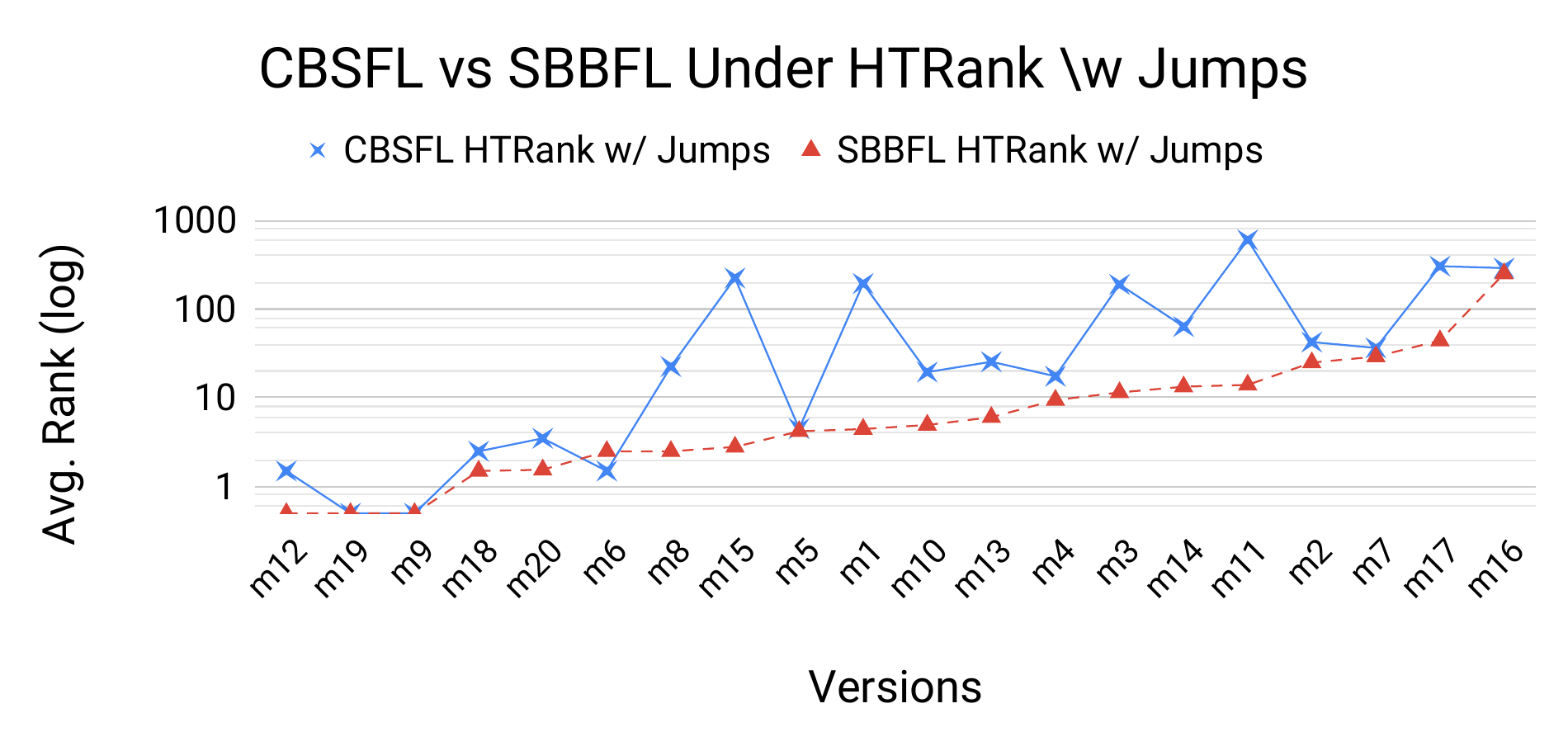
Table IV details the fault localization performance we observed for CBSFL and SBBFL under the Standard Rank Score and \(\textrm{HT}_{\textrm{Rank}}\) using six different suspiciousness metrics. The results obtained with \(\textrm{HT}_{\textrm{Rank}}\) were substantially different from those obtained with the Standard Rank Score, in terms of absolute ranks and percentage differences (%\(\Delta\)). The mean Standard Rank Score for SBBFL is lower than that for CBSFL for every suspiciousness metric and subject program. By contrast, for some programs and metrics, the mean \(\textrm{HT}_{\textrm{Rank}}\) scores for CBSFL are lower than those for SBBFL. The mean \(\textrm{HT}_{\textrm{Rank}}\) scores are also higher than the mean Standard Rank Scores overall.
Another way to look at the same phenomenon is shown in Figure 5, which displays empirical probability density plots for the program Otto. Each plot compares the performance of CBSFL to SBBFL using a different evaluation method. The top plot uses the Standard Rank Score while the other plot uses \(\textrm{HT}_{\textrm{Rank}}\). As shown in the top plot, the Standard Rank Scores for both CBSFL and SBBFL are concentrated mainly between 0 and 15, with no values over 60. In the \(\textrm{HT}_{\textrm{Rank}}\) plot, by contrast, the scores for both CBSFL and SBBFL are much more widely dispersed. Figure 4 compares CBSFL to SBBFL with respect to average ranks (on a log scale), under the Standard Rank Score (top) and \(\textrm{HT}_{\textrm{Rank}}\) (bottom), for each version of the program Otto. The suspiciousness metric is RelativeF1. The results for \(\textrm{HT}_{\textrm{Rank}}\) are quite distict from those for the Standard Rank Score, with CBSFL showing much more variability under \(\textrm{HT}_{\textrm{Rank}}\).
These results provide confirmation for the theoretical motivation for \(\textrm{HT}_{\textrm{Rank}}\). Recall that one of the problems with the Standard Rank Score is that it does not account for either the differing structures of fault localization reports or differences in report granularity. SBBFL and CBSFL differ in both structure (ranked CFG fragments vs. ranked basic blocks) and granularity (multiple basic blocks vs. lone basic blocks). We expected the Standard Rank Score to unfairly favor SBBFL because it does not account for these differences and that is exactly what we see in Table IV. Under the Standard Rank Score SBBFL outperforms CBSFL on every program using every suspiciousness score.
To be explicit, SBBFL reports ranked CFG fragments, each of which contains multiple basic blocks. Under the Standard Rank Score those fragments are ranked and the score is the rank of the first fragment in which the bug appears. CBSFL will, by contrast, rank each basic block independently. Now, consider the case where SBBFL reports a CFG fragment at rank 1 that contains 10 basic blocks, one of which contains the bug. Suppose CBSFL also reports each of those basic blocks as maximally suspicious. The Standard Rank Score for CBSFL will be 5 while for SBBFL it will be 1. Thus, the Standard Rank Score is unfairly biased toward SBBFL and against CBSFL. This is once again reflected in Table IV. The new metric \(\textrm{HT}_{\textrm{Rank}}\) does not suffer from this problem. As shown in the table and discussed below, SBBFL often but not always outperforms CBSFL under \(\textrm{HT}_{\textrm{Rank}}\), suggesting that the theoretical correction we expect is indeed occurring. We therefore conclude that \(\textrm{HT}_{\textrm{Rank}}\) provides a better metric for comparison when reports differ in structure and granularity.
RQ3: Which kind of fault localization technique performs better, SBBFL or CBSFL?
Referring once again to Table IV, the \(\textrm{HT}_{\textrm{Rank}}\) results indicate that SBBFL often but not always outperformed CBSFL. In particular, when the measure used was Relative F1 (which was found to be the best-performing measure for SBBFL in [9]), SBBFL performed better for all programs but the compiler. However, when Ochiai was used CBSFL outperformed SBBFL, although CBSFL with Relative F1 outperforms CBSFL with Ochiai. This indicates that SBBFL and Relative F1 may be the best combination tested with one caveat. For the compiler, SBBFL never outperforms CBSFL. However, CBSFL also performs very badly on this large program. This indicates that while CBSFL beats SBBFL on this program neither technique is effective at localizing faults in it.
Study Limitations
The purpose of our case study is to illustrate the application of \(\textrm{HT}_{\textrm{Rank}}\). It was not designed to settle controversies about the suspiciousness metrics we employed. Second, this study used real programs and tests but used synthetic bugs. In the future, we intend to provide an automated analysis system that builds upon the Defects4J dataset [52]. Third, our study included a representative but not exhaustive set of suspiciousness metrics [2] and may not generalize to other metrics.
Finally, no user-study was performed to validate the chosen debugging model against actions an actual programmer would take. Although we would have liked to perform such a study at this time, our resources do not permit us to do so. To be conclusive, such a study would need to be large-scale and to utilize professional programmers who are skilled in traditional debugging and are able to spend significant time learning to use SFL techniques with comparable skill.
Discussion
A new, flexible approach to evaluating automatic fault localization techniques was presented. The new \(\textrm{HT}_{\textrm{Rank}}\) Score provides a principled and flexible way of comparing different fault localization techniques. It is robust to differences in granularity and allows complex fault localization reports (such as those produced by SBBFL) to be incorporated. Unlike previous attempts at cross-technique comparison (see Section 12) the final scores are based on the expected number of steps through a Markov model. The model can incorporate both information from the chosen fault localization technique as well as other information available to the programmer (such as the structure of the program). The \(\textrm{HT}_{\textrm{Rank}}\) Score is sensitive to the model used (see Fig 5) and hence the choice of model is important. The choice should be made based on 1) the fault localization technique(s) being evaluated and 2) observations of programmer behavior. Choosing a model after viewing the results (and picking the model that gives the "best" results) leads to a biased outcome.
Recommendations for Researchers
Report both Standard Rank Score and \(\textrm{HT}_{\textrm{Rank}}\) Score.
If evaluating multi-line faults the Steinmann Rank Score (Def. 18) should be used as the basis for defining the \(\textrm{HT}_{\textrm{Rank}}\) Score.
Report which model is being used and why it was chosen, and include a description of the model.
In the absence of user study data, set \(p_{\text{jump}} = .5\) and set the weights in \({\bf J}\) uniformly.
By evaluating fault localization methods with \(\textrm{HT}_{\textrm{Rank}}\) in addition to the Standard Rank Score researchers will be able to make valid cross-technique comparisons. This will enable the community to better understand the relationships between techniques and report-granularity while taking into account potential programmer behavior during debugging.
Acknowledgement
This work was partially supported by NSF award CCF-1525178 to Case Western Reserve University.
Markov Chain Definitions
Definition. CBSFL Ranked List Markov Chain
To construct a Markov chain representing a list of program locations ranked in descending order by their suspiciousness scores:
Let \(L\) be the set of locations in the program.
For a location \(l \in L\) let \(s(l)\) be its CBSFL suspiciousness score.
Partition the locations in \(L\) into a list of groups \(G = \left\{ g_1 \subseteq L, g_2 \subseteq L, ..., g_n \subseteq L \right\}\) such that for each group \(g_i\) all of the locations it contains have the same score: \( \forall ~ {g_i \in G}, ~ \forall ~ {l, l' \in g_i} \left[ s(l) = s(l') \right]\)
The score of a group \(s(g_i)\) is defined to be the common score of its members: \( \forall ~ {l \in g_i} \left[ s(g_i) = s(l) \right]\)
Order \(G\) by the scores of its groups, such that \(g_0\) has the highest score and \(g_n\) has the lowest: \(s(g_0) > s(g_1) > ... > s(g_n)\)
Now construct the set of states. There is one state for each group \(g \in G\) and for each location \(l \in L\). \[S = \left\{ g : g \in G \right\} \cup \left\{ l : l \in L \right\}\]
Finally construct the transition matrix \({\bf P}\) for the states \(S\). \[{\bf P}_{i,j} = \left\{ \begin{array}{lll} 1 & \text{if} & s_i \in L \wedge s_j \in G \wedge s_i \in s_j \\ \\ \frac{{{\left|{L}\right|}} - 1}{2{{\left|{L}\right|}}} & \text{if} & s_i = g_0 \wedge s_j = s_i \\ \\ \frac{1}{2{{\left|{L}\right|}}} & \text{if} & s_i = g_n \wedge s_j = s_i \\ \\ \frac{{{\left|{L}\right|}} - 1}{2{{\left|{L}\right|}}} & \text{if} & s_i \in G \wedge s_j \in G \wedge s_i - 1 = s_j \\ \\ \frac{1}{2{{\left|{L}\right|}}} & \text{if} & s_i \in G \wedge s_j \in G \wedge s_i + 1 = s_j \\ \\ \frac{1}{2{{\left|{s_i}\right|}}} & \text{if} & s_i \in G \wedge s_j \in L \wedge s_j \in s_i \\ \\ 0 & \text{otherwise} \end{array} \right.\]
Definition. CBSFL with Jumps Markov Chain
This definition augments Definition 28.
Let \({\bf J}\) be a "jump" matrix representing ways a programmer might move through the program during debugging.
If \({\bf J}_{x,y} > 0\) then locations \(x,y \in L\) are "connected" by \({\bf J}\).
Let \(p_{\text{jump}}\) be the probability that when visiting a location \(l \in L\) the Markov process "jumps" to another location. Let \(1 - p_{\text{jump}}\) be the probability that the process returns to the state which represents its group instead of jumping. As \(p_\text{{jump}} \rightarrow 0\) the behavior of the chain approaches the behavior of the chain in Definition 28.
The new transition matrix \({\bf P}\) for the states \(S\) is
\[\begin{aligned} {\bf P}_{i,j} &= \left\{ \begin{array}{cll} 1 - p_{\text{jump}} & \text{if} & s_i \in L \wedge s_j \in G \wedge s_i \in s_j \\ & & \wedge \left( \sum_{k}{{\bf J}_{i,k}} \right) > 0 \\ \\ p_{\text{jump}} \left( \frac{{\bf J}_{i,j}}{\sum_{k}{{\bf J}_{i,k}}} \right) & \text{if} & s_i \in L \wedge s_j \in L \wedge {\bf J}_{i,j} > 0 \\ \\ \frac{{{\left|{L}\right|}} - 1}{2{{\left|{L}\right|}}} & \text{if} & s_i = g_0 \wedge s_j = s_i \\ \\ \frac{1}{2{{\left|{L}\right|}}} & \text{if} & s_i = g_n \wedge s_j = s_i \\ \\ \frac{{{\left|{L}\right|}} - 1}{2{{\left|{L}\right|}}} & \text{if} & s_i \in G \wedge s_j \in G \wedge s_i - 1 = s_j \\ \\ \frac{1}{2{{\left|{L}\right|}}} & \text{if} & s_i \in G \wedge s_j \in G \wedge s_i + 1 = s_j \\ \\ \frac{1}{2{{\left|{s_i}\right|}}} & \text{if} & s_i \in G \wedge s_j \in L \wedge s_j \in s_i \\ \\ 0 & \text{otherwise} \end{array} \right. \end{aligned}\]
Definition. Suspicious Behavior Markov Chain
A chain that models a ranked list of suspicious subgraphs:
Let \(H\) be a set of suspicious subgraphs (behaviors).
For a subgraph \(h \in H\) let \(\varsigma(h)\) be its suspiciousness score [9].
Let \(L\) be the set of locations in the program.
Partition the subgraphs in \(H\) into a list of groups \(G = \left\{ g_1 \subseteq H, g_2 \subseteq H, ..., g_n \subseteq H \right\}\) such that for each group \(g_i\) all of the locations in \(g_i\) have the same score: \(\forall ~ {g_i \in G} ~ \forall ~ {a, b \in g_i} \left[ \varsigma(a) = \varsigma(b) \right]\)
Let the score of a group \(\varsigma(g_i)\) be the same as the scores of its members: \( \forall ~ {g_i \in G} ~ \forall ~ {h \in g_i} \left[ \varsigma(g_i) = \varsigma(h) \right]\)
Order \(G\) by the scores of its groups, such that \(g_0\) has the highest score and \(g_n\) has the lowest: \( \varsigma(g_0) > \varsigma(g_1) > ... > \varsigma(g_n)\)
Now construct the set of states. One state for each group \(g \in G\), one state for each subgraph \(h \in H\), and one state for each location \(l \in V_{h}\) for all \(h \in H\). \[S = \left\{ g : g \in G \right\} \cup \left\{ h : h \in H \right\} \cup \left\{ l : l \in V_h,~ \forall~ h \in H \right\}\]
Let \(c: L \rightarrow \mathbb{N}^{+}\) be a function that gives the number of subgraphs \(h \in H\) which a location \(l\) appears in.
Finally construct the transition matrix \({\bf P}\) for the states \(S\). \[{\bf P}_{i,j} = \left\{ \begin{array}{cll} \frac{1}{c(s_i)} & \text{if} & s_i \in L \wedge s_j \in H \wedge s_i \in V_{s_j} \\ \\ \frac{1}{2}\frac{1}{{{\left|{V_{s_i}}\right|}}} & \text{if} & s_i \in H \wedge s_j \in L \wedge s_j \in V_{s_i} \\ \\ \frac{1}{2} & \text{if} & s_i \in H \wedge s_j \in G \wedge s_i \in s_j \\ \\ \frac{{{\left|{H}\right|}} - 1}{2{{\left|{H}\right|}}} & \text{if} & s_i = g_0 \wedge s_j = s_i \\ \\ \frac{1}{2{{\left|{H}\right|}}} & \text{if} & s_i = g_n \wedge s_j = s_i \\ \\ \frac{{{\left|{H}\right|}} - 1}{2{{\left|{H}\right|}}} & \text{if} & s_i \in G \wedge s_j \in G \wedge s_i - 1 = s_j \\ \\ \frac{1}{2{{\left|{H}\right|}}} & \text{if} & s_i \in G \wedge s_j \in G \wedge s_i + 1 = s_j \\ \\ \frac{1}{2{{\left|{s_i}\right|}}} & \text{if} & s_i \in G \wedge s_j \in H \wedge s_j \in s_i \\ \\ 0 & \text{otherwise} \end{array} \right.\]
References
[1] J. Jones, M. Harrold, and J. Stasko, "Visualization of test information to assist fault localization," Proceedings of the 24th International Conference on Software Engineering. ICSE 2002, 2002, doi:10.1145/581339.581397.
[2] Lucia, D. Lo, L. Jiang, F. Thung, and A. Budi, "Extended comprehensive study of association measures for fault localization," Journal of Software: Evolution and Process, vol. 26, no. 2, pp. 172-219, Feb. 2014, doi:10.1002/smr.1616.
[3] S.-F. Sun and A. Podgurski, "Properties of Effective Metrics for Coverage-Based Statistical Fault Localization," in 2016 ieee international conference on software testing, verification and validation (icst), 2016, pp. 124-134, doi:10.1109/ICST.2016.31.
[4] J. A. Jones and M. J. Harrold, "Empirical Evaluation of the Tarantula Automatic Fault-localization Technique," in Proceedings of the 20th ieee/acm international conference on automated software engineering, 2005, pp. 273-282, doi:10.1145/1101908.1101949.
[5] S. Pearson, J. Campos, R. Just, G. Fraser, R. Abreu, M. D. Ernst, D. Pang, and B. Keller, "Evaluating and Improving Fault Localization," in Proceedings of the 39th international conference on software engineering, 2017, pp. 609-620, doi:10.1109/ICSE.2017.62.
[6] C. Parnin and A. Orso, "Are Automated Debugging Techniques Actually Helping Programmers?" in ISSTA, 2011, pp. 199-209.
[7] M. Renieres and S. Reiss, "Fault localization with nearest neighbor queries," in 18th ieee international conference on automated software engineering, 2003. proceedings., 2003, pp. 30-39, doi:10.1109/ASE.2003.1240292.
[8] H. Cheng, D. Lo, Y. Zhou, X. Wang, and X. Yan, "Identifying Bug Signatures Using Discriminative Graph Mining," in Proceedings of the eighteenth international symposium on software testing and analysis, 2009, pp. 141-152, doi:10.1145/1572272.1572290.
[9] T. A. D. Henderson and A. Podgurski, "Behavioral Fault Localization by Sampling Suspicious Dynamic Control Flow Subgraphs," in IEEE conference on software testing, validation and verification, 2018.
[10] G. G. K. Baah, A. Podgurski, and M. J. M. Harrold, "Causal inference for statistical fault localization," in Proceedings of the 19th international symposium on software testing and analysis, 2010, pp. 73-84, doi:10.1145/1831708.1831717.
[11] C. C. Aggarwal and J. Han, Eds., Frequent Pattern Mining. Cham: Springer International Publishing, 2014.
[12] R. Agrawal, T. Imieliński, and A. Swami, "Mining association rules between sets of items in large databases," ACM SIGMOD Record, vol. 22, no. 2, pp. 207-216, Jun. 1993, doi:10.1145/170036.170072.
[13] X. Yan and J. Han, "gSpan: graph-based substructure pattern mining," in 2002 ieee international conference on data mining, 2002. proceedings., 2002, pp. 721-724, doi:10.1109/ICDM.2002.1184038.
[14] C. C. Aggarwal, M. A. Bhuiyan, and M. A. Hasan, "Frequent Pattern Mining Algorithms: A Survey," in Frequent pattern mining, Cham: Springer International Publishing, 2014, pp. 19-64.
[15] X. Yan, H. Cheng, J. Han, and P. S. Yu, "Mining Significant Graph Patterns by Leap Search," in Proceedings of the 2008 acm sigmod international conference on management of data, 2008, pp. 433-444, doi:10.1145/1376616.1376662.
[16] R. Abreu, P. Zoeteweij, and A. Van Gemund, "An Evaluation of Similarity Coefficients for Software Fault Localization," in 2006 12th pacific rim international symposium on dependable computing (prdc'06), 2006, pp. 39-46, doi:10.1109/PRDC.2006.18.
[17] R. Abreu, P. Zoeteweij, R. Golsteijn, and A. J. C. van Gemund, "A practical evaluation of spectrum-based fault localization," Journal of Systems and Software, vol. 82, no. 11, pp. 1780-1792, 2009, doi:10.1016/j.jss.2009.06.035.
[18] P. Agarwal and A. P. Agrawal, "Fault-localization Techniques for Software Systems: A Literature Review," SIGSOFT Softw. Eng. Notes, vol. 39, no. 5, pp. 1-8, Sep. 2014, doi:10.1145/2659118.2659125.
[19] W. E. Wong, R. Gao, Y. Li, R. Abreu, and F. Wotawa, "A Survey on Software Fault Localization," IEEE Transactions on Software Engineering, vol. 42, no. 8, pp. 707-740, Aug. 2016, doi:10.1109/TSE.2016.2521368.
[20] A. Zeller, "Yesterday, My Program Worked. Today, It Does Not. Why?" SIGSOFT Softw. Eng. Notes, vol. 24, no. 6, pp. 253-267, Oct. 1999, doi:10.1145/318774.318946.
[21] F. Tip, "A survey of program slicing techniques," Journal of programming languages, vol. 3, no. 3, pp. 121-189, 1995.
[22] X. Mao, Y. Lei, Z. Dai, Y. Qi, and C. Wang, "Slice-based statistical fault localization," Journal of Systems and Software, vol. 89, no. 1, pp. 51-62, 2014, doi:10.1016/j.jss.2013.08.031.
[23] A. Marcus, A. Sergeyev, V. Rajlieh, and J. I. Maletic, "An information retrieval approach to concept location in source code," Proceedings - Working Conference on Reverse Engineering, WCRE, pp. 214-223, 2004, doi:10.1109/WCRE.2004.10.
[24] J. Zhou, H. Zhang, and D. Lo, "Where should the bugs be fixed? More accurate information retrieval-based bug localization based on bug reports," Proceedings - International Conference on Software Engineering, pp. 14-24, 2012, doi:10.1109/ICSE.2012.6227210.
[25] T.-D. B. Le, R. J. Oentaryo, and D. Lo, "Information retrieval and spectrum based bug localization: better together," in Proceedings of the 2015 10th joint meeting on foundations of software engineering - esec/fse 2015, 2015, pp. 579-590, doi:10.1145/2786805.2786880.
[26] S. Artzi, J. Dolby, F. Tip, and M. Pistoia, "Directed Test Generation for Effective Fault Localization," in Proceedings of the 19th international symposium on software testing and analysis, 2010, pp. 49-60, doi:10.1145/1831708.1831715.
[27] S. K. Sahoo, J. Criswell, C. Geigle, and V. Adve, "Using likely invariants for automated software fault localization," in Proceedings of the eighteenth international conference on architectural support for programming languages and operating systems, 2013, vol. 41, p. 139, doi:10.1145/2451116.2451131.
[28] A. Perez, R. Abreu, and A. Riboira, "A Dynamic Code Coverage Approach to Maximize Fault Localization Efficiency," J. Syst. Softw., vol. 90, pp. 18-28, Apr. 2014, doi:10.1016/j.jss.2013.12.036.
[29] H. Agrawal, J. Horgan, S. London, and W. Wong, "Fault localization using execution slices and dataflow tests," in Proceedings of sixth international symposium on software reliability engineering. issre'95, 1995, pp. 143-151, doi:10.1109/ISSRE.1995.497652.
[30] H. Cleve and A. Zeller, "Locating causes of program failures," Proceedings of the 27th international conference on Software engineering - ICSE '05, p. 342, 2005, doi:10.1145/1062455.1062522.
[31] S. Horwitz, "Identifying the Semantic and Textual Differences Between Two Versions of a Program," SIGPLAN Not., vol. 25, no. 6, pp. 234-245, Jun. 1990, doi:10.1145/93548.93574.
[32] E. Wong, T. Wei, Y. Qi, and L. Zhao, "A Crosstab-based Statistical Method for Effective Fault Localization," in 2008 international conference on software testing, verification, and validation, 2008, pp. 42-51, doi:10.1109/ICST.2008.65.
[33] D. Landsberg, H. Chockler, D. Kroening, and M. Lewis, "Evaluation of Measures for Statistical Fault Localisation and an Optimising Scheme," in International conference on fundamental approaches to software engineering, 2015, vol. 9033, pp. 115-129, doi:10.1007/978-3-662-46675-9.
[34] Y. Zheng, Z. Wang, X. Fan, X. Chen, and Z. Yang, "Localizing multiple software faults based on evolution algorithm," Journal of Systems and Software, vol. 139, pp. 107-123, 2018, doi:10.1016/j.jss.2018.02.001.
[35] C. Liu, L. Fei, X. Yan, J. Han, and S. P. Midkiff, "Statistical debugging: A hypothesis testing-based approach," IEEE Transactions on Software Engineering, vol. 32, no. 10, pp. 831-847, Oct. 2006, doi:10.1109/TSE.2006.105.
[36] J. Ferrante, K. J. Ottenstein, and J. D. Warren, "The program dependence graph and its use in optimization," vol. 9. pp. 319-349, Jul-1987.
[37] S. Ali, J. H. Andrews, T. Dhandapani, and W. Wang, "Evaluating the Accuracy of Fault Localization Techniques," 2009 IEEE/ACM International Conference on Automated Software Engineering, pp. 76-87, 2009, doi:10.1109/ASE.2009.89.
[38] S. Moon, Y. Kim, M. Kim, and S. Yoo, "Ask the Mutants: Mutating faulty programs for fault localization," Proceedings - IEEE 7th International Conference on Software Testing, Verification and Validation, ICST 2014, pp. 153-162, 2014, doi:10.1109/ICST.2014.28.
[39] C. Liu, H. Yu, P. S. Yu, X. Yan, H. Yu, J. Han, and P. S. Yu, "Mining Behavior Graphs for ‘Backtrace' of Noncrashing Bugs," in Proceedings of the 2005 siam international conference on data mining, 2005, pp. 286-297, doi:10.1137/1.9781611972757.26.
[40] G. Di Fatta, S. Leue, and E. Stegantova, "Discriminative Pattern Mining in Software Fault Detection," in Proceedings of the 3rd international workshop on software quality assurance, 2006, pp. 62-69, doi:10.1145/1188895.1188910.
[41] F. Eichinger, K. Böhm, and M. Huber, "Mining Edge-Weighted Call Graphs to Localise Software Bugs," in European conference machine learning and knowledge discovery in databases, 2008, pp. 333-348, doi:10.1007/978-3-540-87479-9_40.
[42] F. Eichinger, K. Krogmann, R. Klug, and K. Böhm, "Software-defect Localisation by Mining Dataflow-enabled Call Graphs," in Proceedings of the 2010 european conference on machine learning and knowledge discovery in databases: Part i, 2010, pp. 425-441.
[43] Z. Mousavian, M. Vahidi-Asl, and S. Parsa, "Scalable Graph Analyzing Approach for Software Fault-localization," in Proceedings of the 6th international workshop on automation of software test, 2011, pp. 15-21, doi:10.1145/1982595.1982599.
[44] F. Eichinger, C. Oßner, and K. Böhm, "Scalable software-defect localisation by hierarchical mining of dynamic call graphs," Proceedings of the 11th SIAM International Conference on Data Mining, SDM 2011, no. c, pp. 723-734, 2011.
[45] S. Parsa, S. A. Naree, and N. E. Koopaei, "Software Fault Localization via Mining Execution Graphs," in Proceedings of the 2011 international conference on computational science and its applications - volume part ii, 2011, pp. 610-623.
[46] L. Mariani, F. Pastore, and M. Pezze, "Dynamic Analysis for Diagnosing Integration Faults," IEEE Trans. Softw. Eng., vol. 37, no. 4, pp. 486-508, Jul. 2011, doi:10.1109/TSE.2010.93.
[47] A. Yousefi and A. Wassyng, "A Call Graph Mining and Matching Based Defect Localization Technique," in 2013 ieee sixth international conference on software testing, verification and validation workshops, 2013, pp. 86-95, doi:10.1109/ICSTW.2013.17.
[48] J. P. A. Ioannidis, "Why most published research findings are false," PLoS Medicine, vol. 2, no. 8, pp. 0696-0701, 2005, doi:10.1371/journal.pmed.0020124.
[49] C. M. Grinstead and J. L. Snell, Introduction to Probability, 2nd ed. Providence, RI: American Mathematical Society, 1997.
[50] J. G. Kemeny and J. L. Snell, Finite Markov Chains, First. Princeton, NJ: Van Nostrand, 1960.
[51] T. A. Davis, "Algorithm 832: UMFPACK V4.3—an Unsymmetric-pattern Multifrontal Method," ACM Trans. Math. Softw., vol. 30, no. 2, pp. 196-199, Jun. 2004, doi:10.1145/992200.992206.
[52] R. Just, D. Jalali, and M. D. Ernst, "Defects4J: A Database of Existing Faults to Enable Controlled Testing Studies for Java Programs," in Proceedings of the 2014 international symposium on software testing and analysis, 2014, pp. 437-440, doi:10.1145/2610384.2628055.
[53] F. Steimann, M. Frenkel, and R. Abreu, "Threats to the validity and value of empirical assessments of the accuracy of coverage-based fault locators," Proceedings of the 2013 International Symposium on Software Testing and Analysis - ISSTA 2013, p. 314, 2013, doi:10.1145/2483760.2483767.
Jones et al. did not use the term "suspiciousness score" or "suspiciousness metric" in their 2002 paper [1]. They introduced the term "suspiciousness score" in their 2005 paper [4], in the context of ranking statements. Both terms are now in common use.↩
A dependence sphere is computed from the Program Dependence Graph (PDG) [31], [36]. In a PDG, program elements are nodes and their control and data dependencies are represented as edges. Given two nodes \(\alpha\) and \(\beta\) a graph with a shortest path (ignoring edge directionality) \(\pi\) between them, the sphere is all those nodes in the graph have have a path from \(\alpha\) as short (or shorter) than \(\pi\) (once again ignoring edge directionality).↩
Implementations of these two computations maybe found in
https://github.com/timtadh/expected-hitting-times.↩See https://hackthology.com/pdfs/scam-2019-supplement.pdf↩