Behavioral Fault Localization by Sampling Suspicious Dynamic Control Flow Subgraphs
Tim A. D. Henderson and Andy Podgurski.
Behavioral Fault Localization by Sampling Suspicious Dynamic Control Flow
Subgraphs. ICST 2018.
DOI.
PDF.
WEB.
Abstract
We present a new algorithm, Score Weighted Random Walks (SWRW), for behavioral fault localization. Behavioral fault localization localizes faults (bugs) in programs to a group of interacting program elements such as basic blocks or functions. SWRW samples suspicious (or discriminative) subgraphs from basic-block level dynamic control flow graphs collected during the execution of passing and failing tests. The suspiciousness of a subgraph may be measured by any one of a family of new metrics adapted from probabilistic formulations of existing coverage-based statistical fault localization metrics. We conducted an empirical evaluation of SWRW with nine subgraph-suspiciousness measures on five real-world subject programs. The results indicate that SWRW outperforms previous fault localization techniques based on discriminative subgraph mining.
Introduction
Automated fault localization techniques have been developed to help programmers locate software faults (bugs) responsible for observed software failures. Many of these techniques are statistical in nature (e.g., {Jones 2002, Liblit 2005, Liu 2005}). They employ statistical measures of the association, if any, between the occurrence of failures and the execution of particular program elements like statements or conditional branches. The program elements that are most strongly associated with failures are identified as "suspicious", so that developers can examine them to see if they are faulty. The association measures that are used are often called suspiciousness metrics {Jones 2004}. Such statistical fault localization (SFL) techniques typically require execution profiles (or spectra) and PASS/FAIL labels for a set of both passing and failing program runs. Each profile entry characterizes the execution of a particular program element during a run. For example, a statement-coverage profile for a run indicates which statements were executed at least once. The profiles are collected with program instrumentation, while the labels are typically supplied by software testers or end users.
Coverage Based Statistical Fault Localization (CBSFL) techniques compute a suspiciousness score for each program element. The elements are presented to the programmer as a ranked list with the most suspicious elements at the top {Liblit 2005}. Programmers utilize the list to guide their debugging effort by starting at the most suspicious element and moving down. The effectiveness of a CBSFL suspiciousness metric is judged by how accurately it ranks a bug's (or bugs) location in a program. The higher in the list the bug's location appears the better the metric performs {Lucia 2014}.
Kochhar et al. {Kochhar 2016} recently surveyed 386 software engineering practitioners about their expectations for automated fault localization. While practitioners indicated their preference for very accurate algorithms, over 85% of respondents also indicated their preference for tools which help them understand the output of fault localization algorithms. This is an important finding as most statistical approaches do not provide an explanation of their results. The SFL techniques often simply compute suspiciousness measures and rank the program elements accordingly. These rankings may be helpful, but without more information programmers could overlook the faulty element even when it is ranked highly.
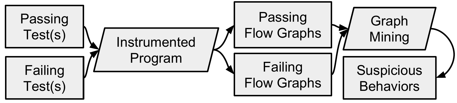
Suspicious-Behavior Based Fault Localization (SBBFL) is a statistical fault localization technique that aids the programmer in understanding suspiciousness scores by providing a context of interacting elements. (NB: Dynamic slicing {Tip 1995} also provides such a context, but does not in itself involve suspiciousness measures) Instead of implicating a single element, SBBFL implicates a larger runtime behavior (see process in Figure 1). The implicated control flow paths (or subgraphs) may help the programmer understand the nature of a bug {Cheng 2009}.
We present a new algorithm, Score-Weighted Random Walks (SWRW), for behavioral fault-localization. SWRW belongs to a family of discriminative graph-mining algorithms that have previously been used for behavioral fault localization { Liu 2005, DiFatta 2006, Eichinger 2008, Cheng 2009, Eichinger 2010, Eichinger 2011, Mousavian 2011, Mariani 2011, Parsa 2011, Yousefi 2013 }. Graph mining is very powerful in principle but algorithms must make trade-offs to address the challenging combinatorics of the graph mining problem. Our new algorithm, SWRW, mitigates the combinatorics by randomly sampling "suspicious" subgraphs from dynamic control flow graphs. During the sampling process, the most suspicious subgraphs (as judged by a suitable suspiciousness metric) are favored for selection. Unlike previous algorithms, SWRW can be used with a wide variety of suspiciousness metrics --- which allows it to use better metrics than available to previous work. Even when using the same metric as similar algorithms, SWRW localizes faults more accurately than they do.
Summary of Contributions
-
A new behavioral fault localization algorithm, SWRW, that samples suspicious subgraphs from dynamic control flow graphs. Unlike similar algorithms, SWRW can be used with a variety of suspiciousness metrics.
-
New generalizations of existing suspiciousness metrics that allow them to be applied to behaviors represented by subgraphs of dynamic control flow graphs.
-
An empirical study whose results suggest that SWRW is more accurate than similar algorithms.
-
Dynagrok, a new instrumentation, mutation, and analysis tool for the Go programming language.
Dynagrok: A New Profiling Tool
All Coverage-Based Statistical Fault Localization (CBSFL) techniques use coverage profiles to gather information on how software behaved when executed on a set of test inputs. A coverage profile typically contains an entry for each program element of a given kind (e.g., statement, basic block, branch, or function), which records whether (and possibly how many times) the element was executed during the corresponding program run. The profiles and PASS/FAIL labels for all tests are then used to compute a statistical suspiciousness score for each program element.
The process of gathering the coverage information from running programs is called profiling and there are many different varieties of profilers and profiling techniques available. Coverage profiling is a simple and widely implemented technique, which is why it has been widely used by the fault localization community. Another technique is tracing, which logs the sequence of program locations as they are executed. The traces provide detailed information on the behavior of the program but could grow to be very large for long running programs. This paper uses execution flow profiling which computes the dynamic interprocedural control flow graph of a program's execution. This provides some of the benefits of tracing without recording an excessive amount of data.
To capture execution flow profiles we developed Dynagrok, a new analysis, instrumentation and mutation platform for the Go programming language. Go is a newer language (2009) from Google that has been seeing increasing adoption in industry. It has been adopted for web programming, systems programming, "DevOps," network programing, and databases {http://tiobe.com/tiobe-index/, http://blog.golang.org/survey2017-results}. Dynagrok builds upon the abstract syntax tree (AST) representation provided by the Go standard library.
Dynagrok collects profiles by inserting instrumentation into the AST of the
subject program. The profiles currently collected are dynamic control flow
graphs (DCFGs) whose vertices represent basic blocks. A basic
block is a sequence of program operations that can only be entered at the
start of the sequence and can only be exited after the last operation in the
sequence
{Aho 2007}.
A basic-block level control flow graph (CFG) is a directed labeled
graph \(g = (V, E, l)\) comprised of a finite set of
vertices \(V\), a set of edges \(E
\subseteq V \times V\), and a labeling function \(l\) mapping vertices and edges to labels. Each vertex
\(v \in V\) represents a basic block of the program.
Each edge \((u, v) \in E\) represents a transition in
program execution from block \(u\) to block \(v\). The labeling function \(l\)
labels the basic blocks with a unique identifier (e.g.
function-name:block-id), which is consistently applied across
multiple executions but is never repeated in the same execution.
Figure 2 shows an example DCFG collected by Dynagrok for a simple program that
computes terms of the Fibonacci sequence. To collect such graphs Dynagrok parses
the program into an AST using Go's standard library. Dynagrok then uses a
custom control flow analysis to build static control flow graphs. Each basic
block holds pointers to the statements inside of the AST. The blocks also have a
pointer to the enclosing lexical block in the AST. Using this information,
Dynagrok inserts profiling instructions into the AST at the beginning of each
basic block. The instructions inserted by Dynagrok use its dgruntime library
to track the control flow of each thread (which is called a goroutine in Go).
When the program shuts down (either normally or abnormally) the dgruntime
library merges the flow graphs from all the threads together and writes out the
result.
(Read the rest of the paper as a pdf)
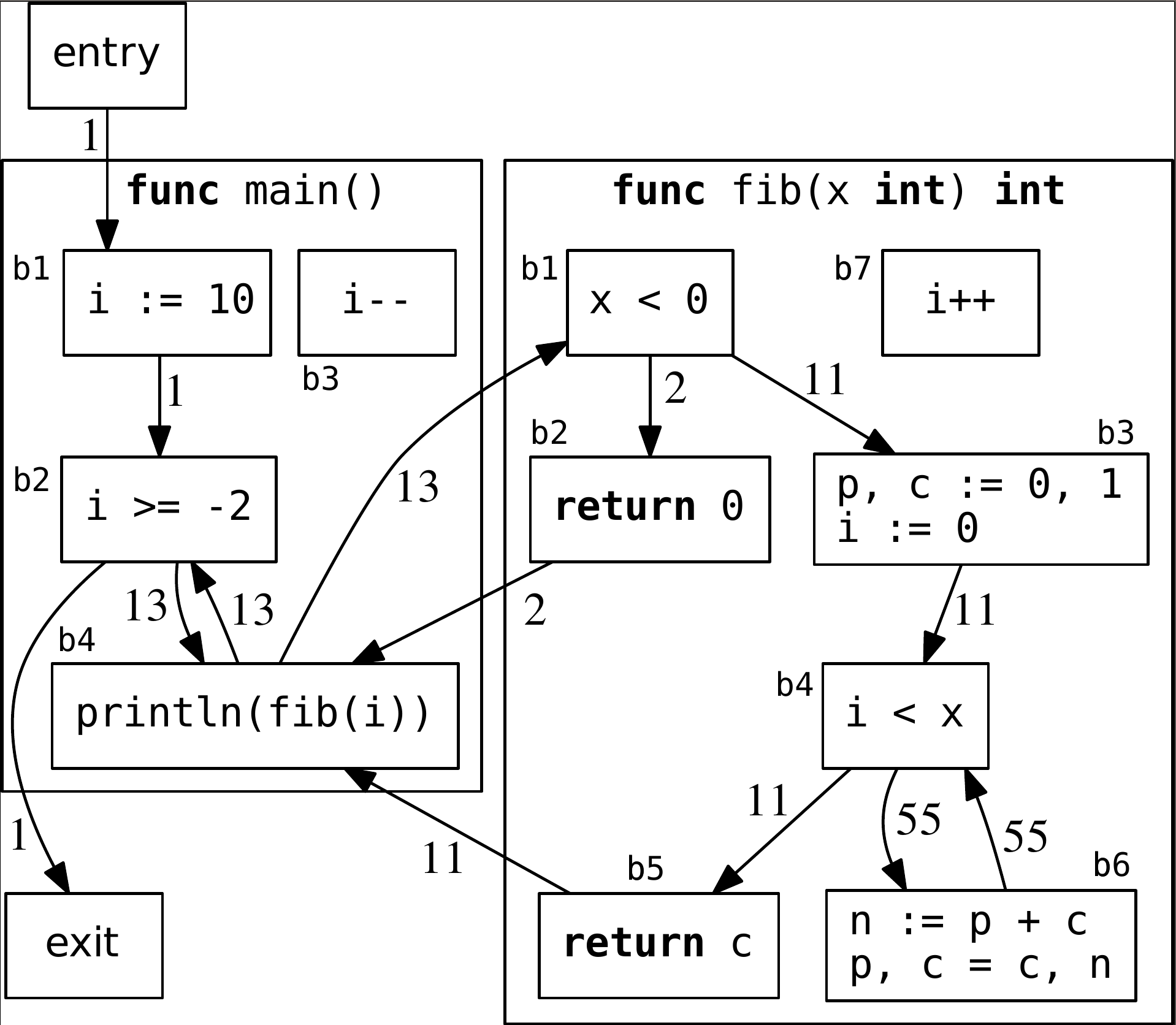
in Listing 1 (see below).
b1) that, in conjunction with the name of the containing function,
serves as the label for the block (e.g. main:b1). Each edge shows
the number of traversals taken during the execution of the program. Note that
the loop update blocks (main:b3 and fib:b7) will not
be in the profiles because Dynagrok instruments the Go source code and profiling
instructions cannot be syntactically inserted in those locations. The
instrumented program is shown on the right.
package main

func main() {
    for i := 10; i >= -2; i-- {
        println(fib(i))
    }
}

func fib(x int) int {
    if x < 0 {
        return 0
    }
    p, c := 0, 1
    for i := 0; i < x; i++ {
        n := p + c
        p, c = c, n
    }
    return c
}
package main

import "dgruntime"

func main() {
    defer func() { dgruntime.Shutdown() }()
    dgruntime.EnterFunc("main")
    defer func() { dgruntime.ExitFunc("main") }()
    for i := 10; dgruntime.EnterBlkFromCond(2) && i >= -2; i-- {
        dgruntime.EnterBlk(4)
        println(fib(i))
    }
}

func fib(x int) int {
    dgruntime.EnterFunc("fib")
    defer func() { dgruntime.ExitFunc("fib") }()
    if x < 0 {
        dgruntime.EnterBlk(2)
        return 0
    }
    dgruntime.EnterBlk(3)
    p, c := 0, 1
    for i := 0; dgruntime.EnterBlkFromCond(4) && i < x; i++ {
        dgruntime.EnterBlk(6)
        n := p + c
        p, c = c, n
    }
    dgruntime.EnterBlk(5)
    return c
}