Tim A. D. Henderson, Bobby Dorward, Eric Nickell, Collin Johnston, and Avi Kondareddy. Flake Aware Culprit Finding. ICST Industry Track 2023.
DOI. PDF. WEB. Google Research Preprint.

Note

This is a conversion from a latex paper I wrote. If you want all formatting correct you should read the pdf version.

Abstract

When a change introduces a bug into a large software repository, there is often a delay between when the change is committed and when bug is detected. This is true even when the bug causes an existing test to fail! These delays are caused by resource constraints which prevent the organization from running all of the tests on every change. Due to the delay, a Continuous Integration system needs to locate buggy commits. Locating them is complicated by flaky tests that pass and fail non-deterministically. The flaky tests introduce noise into the CI system requiring costly reruns to determine if a failure was caused by a bad code change or caused by non-deterministic test behavior. This paper presents an algorithm, Flake Aware Culprit Finding, that locates buggy commits more accurately than a traditional bisection search. The algorithm is based on Bayesian inference and noisy binary search, utilizing prior information about which changes are most likely to contain the bug. A large scale empirical study was conducted at Google on 13,000+ test breakages. The study evaluates the accuracy and cost of the new algorithm versus a traditional deflaked bisection search.

Introduction

Fast, collaborative, large scale development is enabled by the use of Continuous Integration in a mono-repository (monorepo) environment where all of the source code is stored in a single shared repository (Potvin and Levenberg 2016). In a monorepo, all developers share a single source of truth for the state of the code and most builds are made from “head” (the most recent commit to the repository) using the source code for all libraries and dependencies rather than versioned pre-compiled archives. This enables (among other things) unified versioning, atomic changes, large scale refactorings, code re-use, cross team collaboration, and flexible code ownership boundaries.

Very large scale monorepos (such as those at Google (Potvin and Levenberg 2016; Memon et al. 2017), Microsoft (Herzig and Nagappan 2015), and Facebook (Machalica et al. 2019)) require advanced systems for ensuring changes submitted to the repository are properly tested and validated. Continuous Integration (CI) (Fowler 2006) is a system and practice of automatically integrating changes into the code repository that serves as the source of truth for the organization. In modern environments, integration involves not only performing the textual merge required to add the change but also verification tasks such as ensuring the software compiles and the automated tests pass both on the new change before it is integrated and after it has been incorporated into the main development branch.

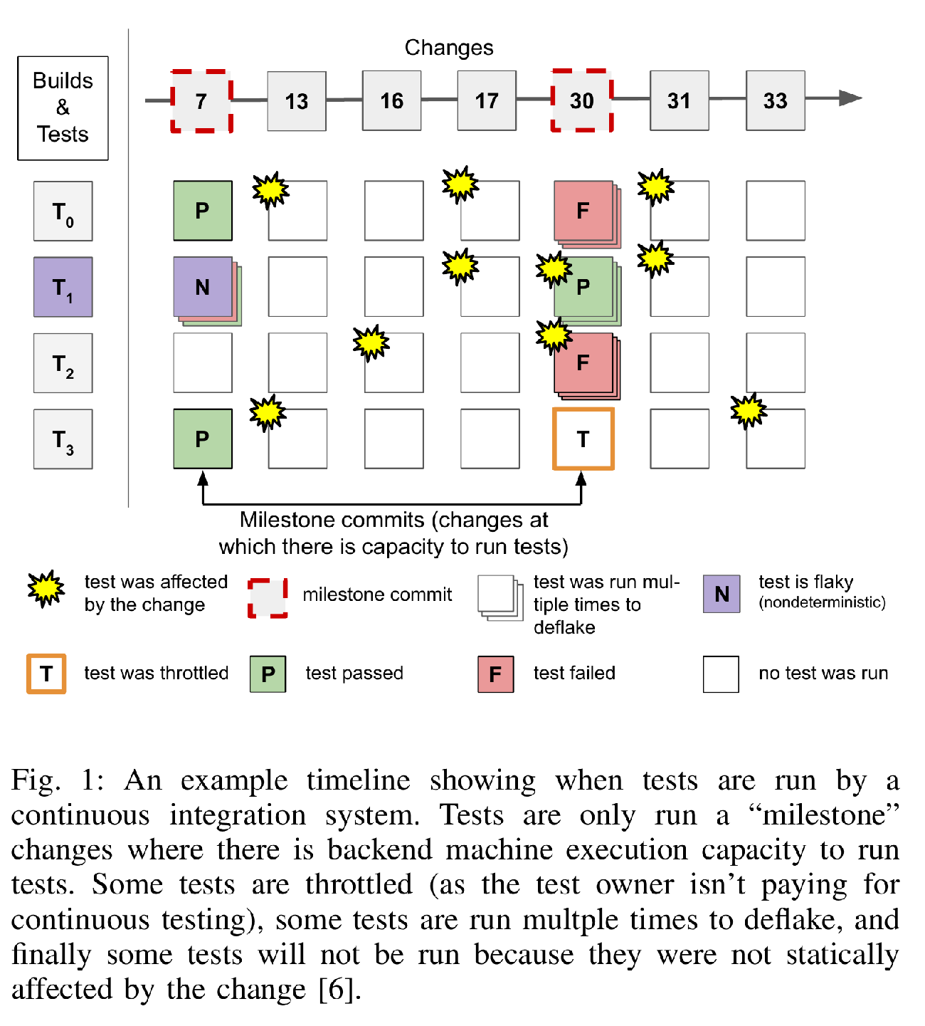
Due to resource constraints, tests are only run at specific versions (called milestones at Google) and many tests may be skipped because they were not affected by the intervening changes (as determined by static build dependencies) (Gupta, Ivey, and Penix 2011). This process is illustrated in Figure [fig:ci-timeline]. A test is considered passing at a version \(b\) if and only if it has a passing result at the most recent preceding affecting version. Formally, if there exists a version \(a\) where the test is passing and \(a \le b\) and there does not exist an intervening version \(c\), \(a < c \le b\), which affects the test then the test is passing at version \(a\). A project’s status is considered passing at a version \(b\) if all tests are passing (using the above definition) at version \(b\).

If a test \(t\) is failing (consistently) at a milestone version \(m\), it may not necessarily mean that version \(m\) introduced a change which broke test \(t\). As shown in Figure [fig:ci-timeline] one or more changes between \(m\) and the previous milestone at which test \(t\) was run may have introduced a breaking change. Figuring out which version introduced the breakage is called culprit finding.

Many companies now employ automated culprit finding systems. These systems typically implement a (possibly n-way) “bisect search” similar to the one built into the Git version control system (Couder 2008). Git’s bisect command runs a binary search on the versions between the first known breaking version and the last known passing version to identify the version which broke the test.

In the Google environment, there are two problems with a traditional bisection algorithm (Couder 2008): (1) it does not account for flaky (non-deterministic) tests, and (2) when using \(k\)-reruns to deflake the search accuracy plateaus while build cost continues to increase linearly. This paper proposes a new method for culprit finding which is both robust to non-deterministic (flaky) test behavior and can identify the culprit with only logarithmic builds in the best case by using prior information to accelerate the search.

Contributions

1. A Flake Aware Culprit Finding (FACF) algorithm.

2. A mathematical model for culprit finding adjusting for non-deterministic test behavior.

3. A large scale empirical study of FACF on Google’s mono repository comparing its performance against the traditional bisect algorithm.

4. The study also evaluates the effectiveness: (a) optimizations for FACF, and (b) adding deflaking runs to Bisect.

Background

At Google, the Test Automation Platform (TAP) runs most tests that can run on a single machine (and do not use the network except for the loopback interface)¹ and can run in under 15 minutes.² Figure [fig:ci-timeline] illustrates at a high level of how TAP works. First, (not illustrated) tests are grouped into logical projects by the teams that own them. Then, (for accounting and quota allocation purposes) those projects are grouped into very high level groupings called Quota Buckets. Each Quota Bucket is scheduled independently when build resources are available. This means that TAP does not run every test at every version. Instead it only runs tests periodically at select versions called “Milestones” (Memon et al. 2017; Micco 2013; Leong et al. 2019).

When scheduling a Milestone, all the tests that are built and run with the same command line flags to the build system³ are grouped into a set. That set is filtered to remove tests that haven’t been affected by a change to themselves or a build level dependency (Gupta, Ivey, and Penix 2011; Micco 2013, 2012). This is a very coarse grained form of static dependence-based test selection (Binkley 1992; Horwitz and Reps 1992; Tip 1995). Google’s use of build dependence test selection has been influential and it is now also used at a number of other corporations who have adopted Bazel or similar tools (Ananthanarayanan et al. 2019; Machalica et al. 2019). Finally, that (potentially very large) set of “affected” tests is sent to the Build System (Wang et al. 2020) which batches them into efficiently sized groups and then builds and runs them when there is capacity.

Since tests are only run periodically even with accurate build level dependence analysis to drive test selection, there are usually multiple changes which may have introduced a fault in the software or a bug in the test. Finding these “bug inducing changes” – which we call culprits – is the subject of this paper. The process of finding these changes is aggravated by any non-deterministic behavior of the tests and the build system running them.

Flaky Tests

When a test behaves non-deterministically, we refer to it, using the standard term, as a flaky test. A flaky test is one that passes or fails non-deterministically with no changes to the code of either the test or the system under test. At Google, we consider all tests to be at least slightly flaky as the machines that tests are running on could fail in ways that get classified as a test failure (such as resource exhaustion due to a noisy neighbor resulting in a test exceeding its time limit). We encourage everyone to adopt this conservative view for the purposes of identifying culprits.

An important input to the culprit finding algorithm we are presenting is an estimate of how flaky a test might be, as represented by an estimated probability of the test failing due to a flaky failure. We will denote the estimated probability of failure due to a flake for a test \(t\) as \(\hat{f}_t\). The actual probability of failure due to a flake will be denoted \(f_t\) (it is impossible in practice to know \(f_t\)). At Google, we estimate \(\hat{f}_t\) based on the historical failure rate of the test. Apple and Facebook recently published on their work in on estimating flake rates (Kowalczyk et al. 2020; Machalica et al. 2020). One challenge with flake rate estimation is that a single change to the code can completely change the flakiness characteristics of a test in unpredictable ways. Making the flake rate estimation sensitive to recent changes is an ongoing challenge and one we partially solve in this work by doing live re-estimation of the flake rate during the culprit finding process itself.

Culprit Finding

Informally, Culprit Finding is the problem of identifying a version \(c\) between two versions \(a\) and \(b\) such that \(a < c \le b\) where a given test \(t\) was passing at \(a\), failing at \(b\), and \(c\) is the version which introduced the fault. At Google we consider the passing status of a test to be 100% reliable and therefore version \(a\) cannot be a culprit but version \(b\) could be the culprit. For simplicity, this paper only considers searching for the culprit for a single test \(t\) (which failed at \(b\)) but in principle it can be extended to a set of tests \(T\).

Google’s version control system, Piper (Potvin and Levenberg 2016), stores the mainline history as a linear list of versions. Each version gets a monotonically, but not sequentially, increasing number as its version number called the Changelist Number or CL number for short. Thus, our implementation and experiments do not consider branches and merges as would be necessary for a Distributed Version Control System (DVCS) such as git. However, only trivial changes to the mathematics are needed to apply our approach to such an environment (Couder 2008).

Thus, the versions larger than \(a\) and smaller or equal to \(b\) are an ordered list of items we will call the search range and denote as \(S = \left\{s_1, ..., s_{n-1}, s_n\right\}\) where \(s_n = b\). During the search, test executions will be run (and may be run in parallel) at various versions. The unordered set of executions at version \(s_i\) will be denoted \(X_i\).

For the purposes of culprit finding, based on the status of failure detected, the build/test execution statuses are mapped to one of 2 possible states: PASS or FAIL. We denote (for version \(s_i\)): the number of statuses that map to PASS as \(\texttt{\small PASSES}(X_i)\) and the number of statuses that map to FAIL as \(\texttt{\small FAILS}(X_i)\).

Bisection

The Bisect algorithm is a specialized form of binary search. It runs tests (or more generally any operation on the code that can return PASS or FAIL) to attempt to identify which commit introduced a bug. Algorithm [alg:bisect] gives the psuedo-code for this procedure. Bisect is now commonly implemented in most version control systems (see git bisect and hg bisect as common examples). In the case of Distributed Version Control Systems (DVCS) systems such as ‘git‘ and ‘hg‘ the implementation of bisect is somewhat more complex as they model version history as a directed acyclic graph (Couder 2008).

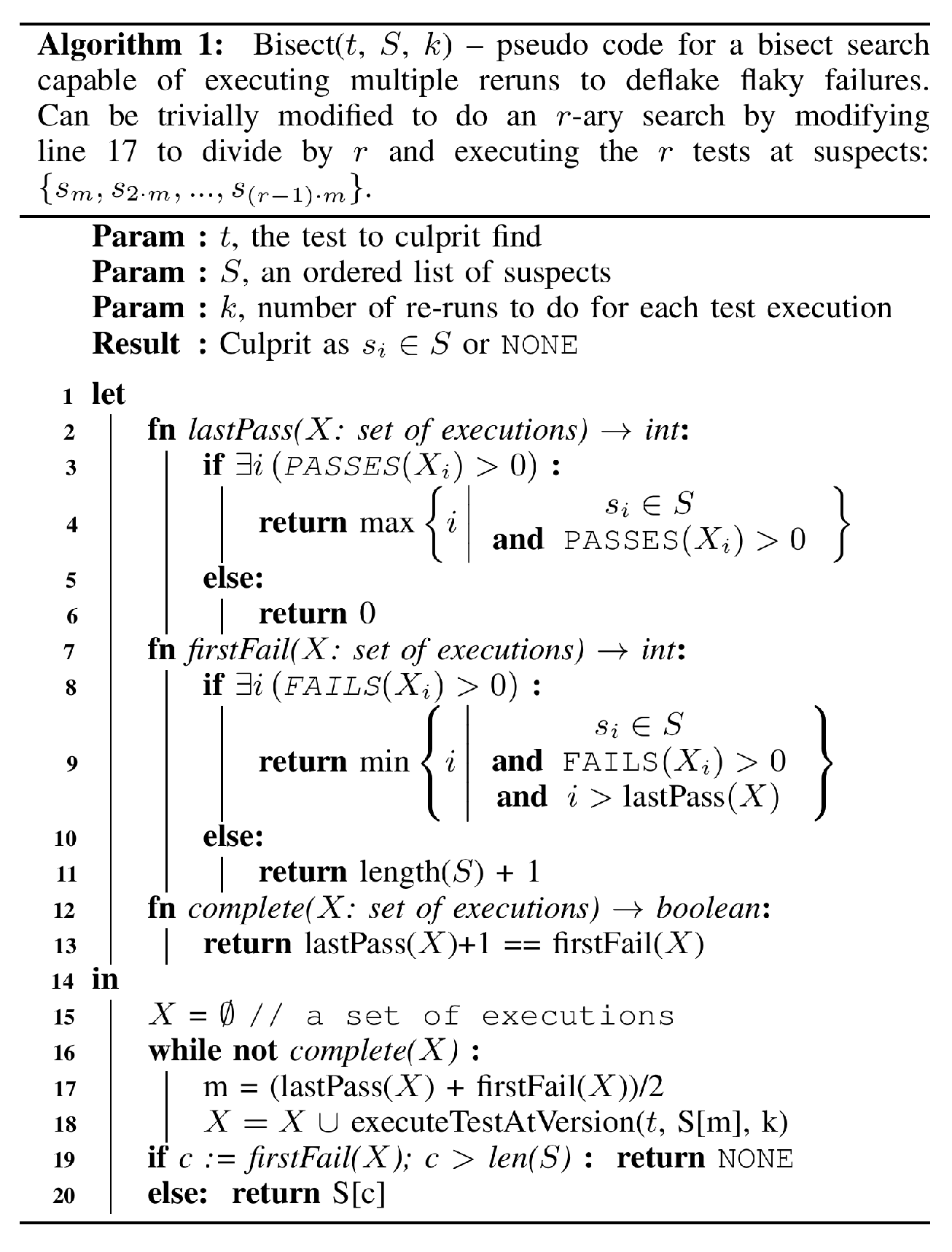
The algorithm presented in Alg [alg:bisect] has two important changes from the standard binary search. First, it takes into account that a test can fail and pass at the same version and the firstFail function specifically looks for a failure after the lastPass. Second, it takes a parameter \(k\) which allows the user to specify that each test execution be run \(k\) times. This allows the user to “deflake” the test executions by rerunning failures. Our empirical evaluation (Section 5) examines both the cost and effectiveness of this simple modification. While this simple modification to bisect may be reasonably effective for moderately flaky tests, it does not explicitly model the effect of non-deterministic failures on the likelihood of a suspect to be the culprit.

Guessing Games and Noisy Searches

One can view the culprit finding scenario as a kind of guessing game. The questioner guesses the test always fails at a given suspect version. A test execution at that suspect acts as a kind of “responder” or “oracle” which answers. The test execution is an unreliable oracle which may answer FAIL when it should have answered PASS. But, the oracle never answers PASS when it should have answered FAIL – note the asymmetry.

This kind of guessing game is a Rényi-Ulam game, which has been well characterized by the community (Pelc 2002). The main differences from the “classical” games presented by Rényi and separately by Ulam is (a) the format of the questions and (b) the limitations placed on the oracle responding incorrectly. In a common formulation of the Rényi-Ulam game, the questioner is trying to “guess the number” between (for instance) 1 and 1,000,000. Each question is allowed to be any subset of numbers in the search range. The responder or oracle is allowed to lie at most a fixed number of times (for instance once or twice). This formulation has allowed the community to find analytic solutions to determine the number of questions in the optimal strategy. We refer the reader to the survey from Pelc for an overview of the field and its connection with error correcting codes (Pelc 2002). The culprit finding scenario is “noisy binary search” scenario where the oracle only lies for one type of response. Rivest et al. (Rivest, Meyer, and Kleitman 1978) provide a theoretical treatment of this “half-lie” variant (as well as the usual variation).

Bayesian Binary Search

Ben Or and Hassidim (Ben-Or and Hassidim 2008) noted the connection between these “Noisy Binary Search” problems and Bayesian inference. Our work builds off of their formulation and applies it to the culprit finding setting. In the Bayesian setting, consider the probability each suspect is the culprit and the probability there is no culprit (i.e. the original failure was caused by a flake). These probabilities together form a distribution: \[(\textrm{Pr}\left[{\text{there is no culprit}}\right]) + \sum_{i=1}^{n} \textrm{Pr}\left[{s_i \text{ is the culprit}}\right] = 1\]

We represent this distribution with \(\textrm{Pr}\left[{C_i}\right]\) with \(i=1..(n+1)\) where \[\begin{aligned} \begin{split} \textrm{Pr}\left[{C_i}\right] &= \textrm{Pr}\left[{s_i \text{ is the culprit}}\right], \; \forall \; i \in [1, n] \\ \textrm{Pr}\left[{C_{n+1}}\right] &= \textrm{Pr}\left[{\text{there is no culprit}}\right] \\ \end{split}\end{aligned}\]

Initially when the original failure is first detected at \(s_n\) and the search range is created, the probability distribution is uniform: \(\textrm{Pr}\left[{C_i}\right] = \frac{1}{(n+1)}\) for all \(i \in [1, n+1]\). Now consider new evidence \(E\) arriving. In the Bayesian model, this would update our probability given this new evidence: \[\begin{aligned} \textrm{Pr}\left[{C_i | E}\right] = \frac{\textrm{Pr}\left[{E | C_i}\right] \cdot \textrm{Pr}\left[{C_i}\right]}{\textrm{Pr}\left[{E}\right]} \label{eq:bayes}\end{aligned}\]

In the above equation, the \(\textrm{Pr}\left[{C_i}\right]\) is the prior probability and the probability \(\textrm{Pr}\left[{C_i | E}\right]\) is the posterior probability. In the culprit finding context, the new evidence is typically newly observed test executions. However, there is no reason we cannot take into account other information as well.

In the Bayesian framework, new evidence is applied iteratively. In each iteration, the prior probability is the posterior probability of the previous iteration. Since multiplication is commutative, multiple pieces of evidence can be applied in any order to arrive at the same posterior probability: \[\begin{aligned} \begin{split} \textrm{Pr}\left[{C_i | E_1, E_2}\right] &= \frac{\textrm{Pr}\left[{E_2 | C_i}\right]}{\textrm{Pr}\left[{E_2}\right]} \frac{\textrm{Pr}\left[{E_1 | C_i}\right]}{\textrm{Pr}\left[{E_1}\right]} \textrm{Pr}\left[{Ci}\right] \\ &= \frac{\textrm{Pr}\left[{E_1 | C_i}\right]}{\textrm{Pr}\left[{E_1}\right]} \frac{\textrm{Pr}\left[{E_2 | C_i}\right]}{\textrm{Pr}\left[{E_2}\right]} \textrm{Pr}\left[{Ci}\right] \end{split}\end{aligned}\]

After the current posterior probability has been calculated, it is used to select the next suspect to execute a test at. In the traditional Bayes approach, the suspect to examine is the one with the maximum posterior probability. However, in the context of a noisy binary search, the suspects are ordered so a PASS at suspect \(s_i\) indicates a PASS at all suspects prior to \(s_i\). Following Ben Or and Hassidim (Ben-Or and Hassidim 2008), we convert the posterior distribution to a cumulative probability distribution and select the first suspect with a cumulative probability \(\geq 0.5\).

Flake Aware Culprit Finding

Now we introduce our algorithm, Flake Aware Culprit Finding (FACF), in the Bayesian framework of Ben Or and Hassidim (Ben-Or and Hassidim 2008). As above, let \(\textrm{Pr}\left[{C_i}\right]\) be the probability that suspect \(s_i\) is the culprit and \(\textrm{Pr}\left[{C_{n+1}}\right]\) be the probability there is no culprit. These probabilities are initialized to some suitable initial distribution such as the uniform distribution.

To update the distribution with new evidence \(E\) in the form of a pass or fail for some suspect \(k\), apply Bayes rule (Equation [eq:bayes]). Note that \(\textrm{Pr}\left[{E}\right]\) can be rewritten by Bayes rule in terms of a sum by marginalizing over the likelihood that each suspect \(j\) could be the culprit: \[\begin{aligned} \textrm{Pr}\left[{E}\right] = \sum_{j=1}^{n} \textrm{Pr}\left[{E | C_j}\right] \textrm{Pr}\left[{C_j}\right]\end{aligned}\]

There are two types of evidence: test executions with state PASS or FAIL at suspect \(i\). We indicate these as the events \(P_i\) and \(F_i\) respectively. The marginalized probability of a PASS at \(i\) given there is a culprit at \(j\) is: \[\begin{aligned} \textrm{Pr}\left[{P_i | C_j}\right] = \begin{cases} 1 - \hat{f}_t & \text{if } i < j \\ 0 & \text{otherwise} \end{cases} \label{eq:pass}\end{aligned}\]

The marginalized probability of a FAIL at \(i\) given there is a culprit at \(j\) is: \[\begin{aligned} \textrm{Pr}\left[{F_i | C_j}\right] = \begin{cases} \hat{f}_t & \text{if } i < j \\ 1 & \text{otherwise} \end{cases} \label{eq:fail}\end{aligned}\]

With Equation [eq:pass], we write a Bayesian update for PASS at suspect \(k\) as the following. Given \[\begin{aligned} \textrm{Pr}\left[{C_i | P_k}\right] = \frac{\textrm{Pr}\left[{P_k | C_i}\right] \textrm{Pr}\left[{C_i}\right]}{ \textrm{Pr}\left[{P_k}\right] }\end{aligned}\]

let \[\begin{aligned} \begin{split} \textrm{Pr}\left[{P_k}\right] &= \sum_{j=1}^{n} \textrm{Pr}\left[{P_k | C_j}\right] \textrm{Pr}\left[{C_j}\right] \\ &= \sum_{j=k+1}^{n} (1 - \hat{f}_t) \textrm{Pr}\left[{C_j}\right] \end{split}\end{aligned}\]

then \[\begin{aligned} \textrm{Pr}\left[{C_i | P_k}\right] = \begin{cases} \frac{(1 - \hat{f}_t) \textrm{Pr}\left[{C_i}\right]}{\textrm{Pr}\left[{P_k}\right]} & \text{if } k < i \\ 0 & \text{otherwise} \\ \end{cases}\end{aligned}\]

The update using Equation [eq:fail] for FAIL at suspect \(k\) is similar. Given \[\begin{aligned} \textrm{Pr}\left[{C_i | F_k}\right] = \frac{\textrm{Pr}\left[{F_k | C_i}\right] \textrm{Pr}\left[{C_i}\right]}{ \sum_{j=1}^{n} \textrm{Pr}\left[{F_k | C_j}\right] \textrm{Pr}\left[{C_j}\right] }\end{aligned}\]

let \[\begin{aligned} \begin{split} \textrm{Pr}\left[{F_k}\right] &= \sum_{j=1}^{n} \textrm{Pr}\left[{F_k | C_j}\right] \textrm{Pr}\left[{C_j}\right] \\ &= \sum_{j=1}^{k} \textrm{Pr}\left[{C_j}\right] + \sum_{j=k+1}^{n} \hat{f}_t \textrm{Pr}\left[{C_j}\right] \end{split}\end{aligned}\]

then \[\begin{aligned} \textrm{Pr}\left[{C_i | F_k}\right] = \begin{cases} \frac{\hat{f}_t \textrm{Pr}\left[{C_i}\right]}{\textrm{Pr}\left[{F_k}\right]} & \text{if } k < i \\ \frac{\textrm{Pr}\left[{C_i}\right]}{\textrm{Pr}\left[{F_k}\right]} & \text{otherwise} \\ \end{cases}\end{aligned}\]

The FACF Algorithm

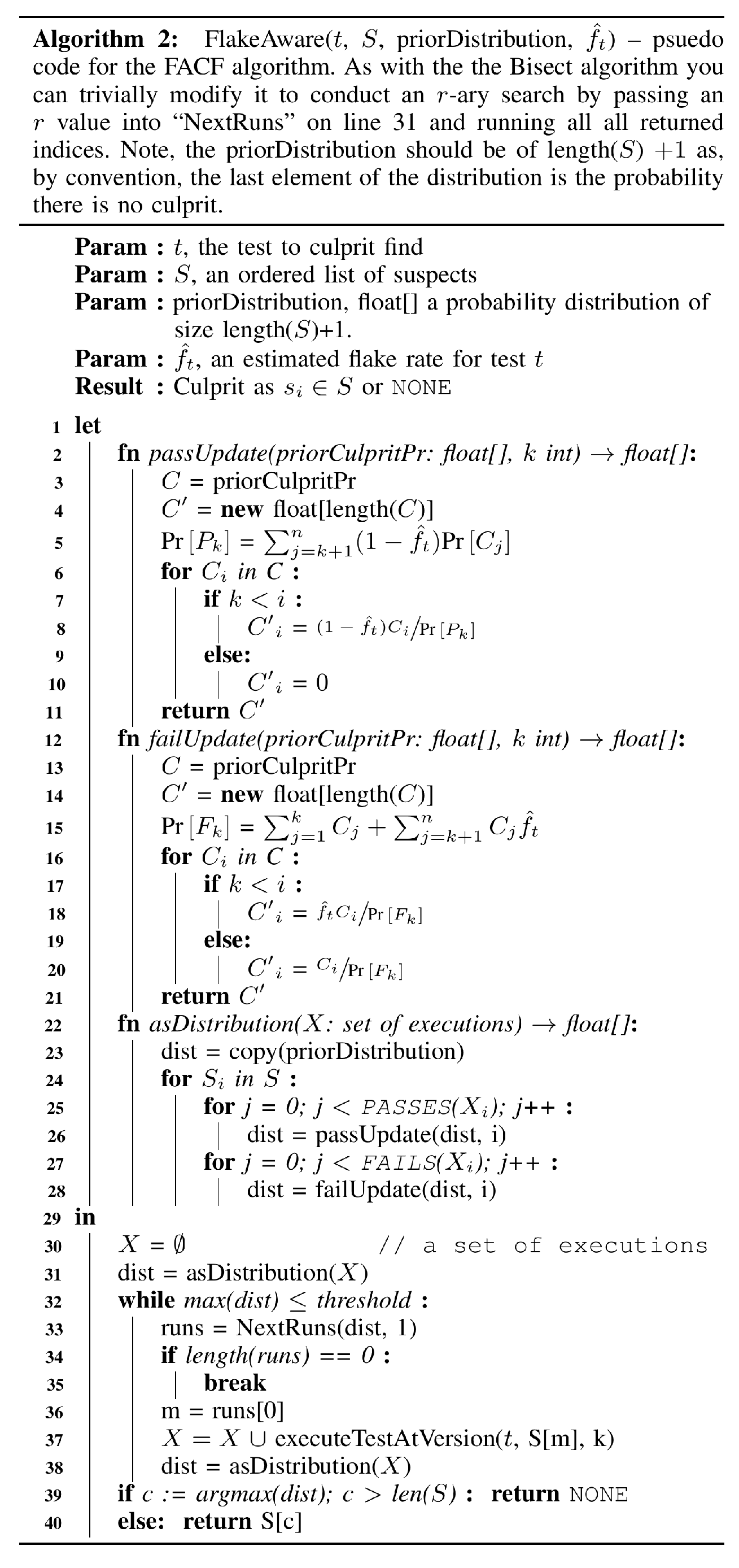
Algorithm [alg:facf] presents the pseudo code for a culprit finding algorithm based on the above Bayesian formulation. It takes a prior distribution (the uniform distribution can be used), an estimated flake rate \(\hat{f}_t\), and the suspects. It returns the most likely culprit or NONE (in the case that it is most likely there is no culprit). The FACF algorithm builds a set of evidence \(X\) containing the observed passes and failures so far. At each step, that evidence is converted to a distribution using the math presented above. Then, FACF calls Algorithm [alg:nextRuns] NextRuns to compute the next suspect to run.

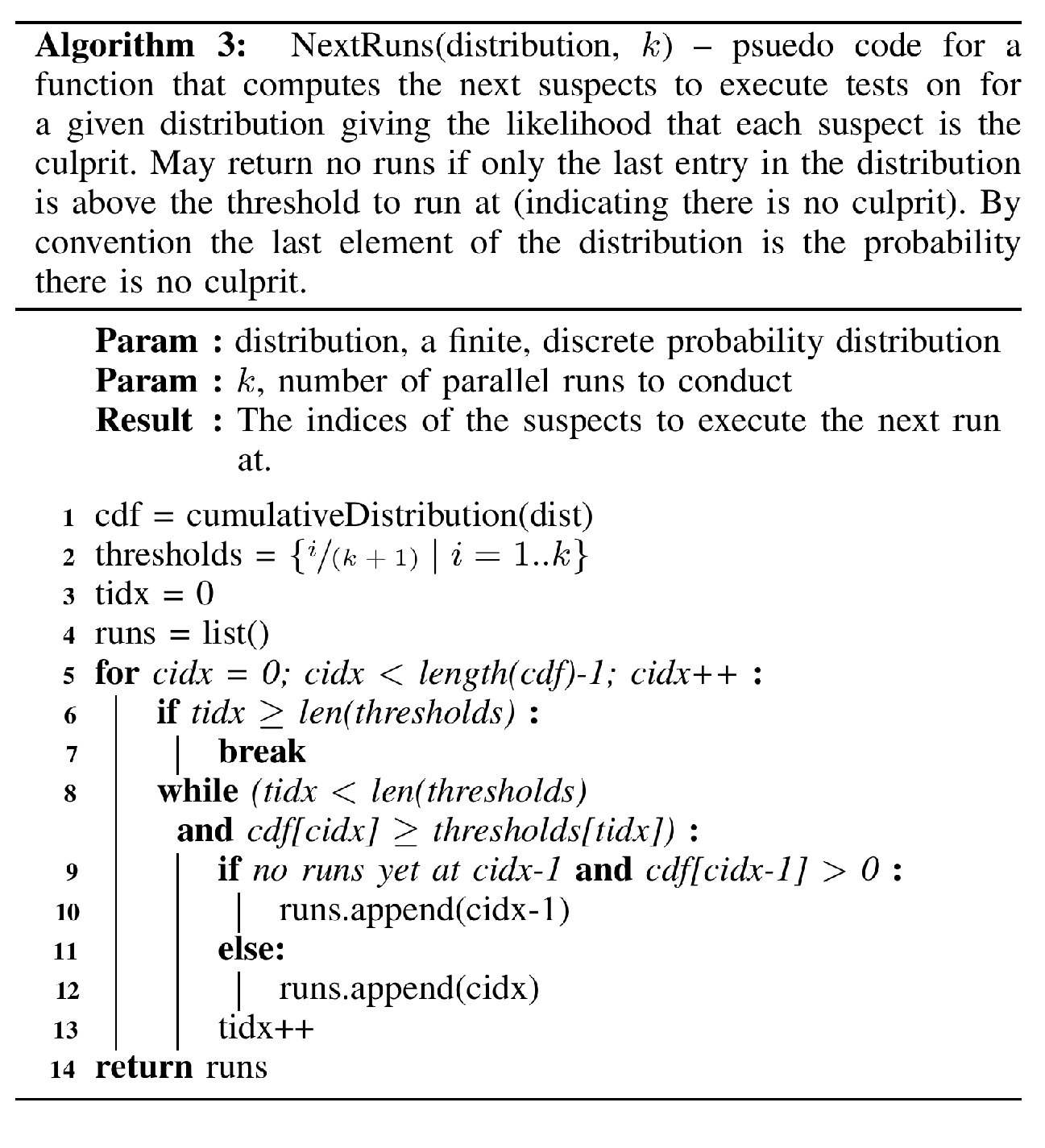
NextRuns converts the probability distribution into a cumulative distribution. It then selects the suspects with cumulative probability over a set of thresholds and returns them. The version of NextRuns we present here has been generalized to allow for \(k\) parallel runs and also contains a minor optimization on lines 10-11. If the suspect \(s_{i-1}\) prior to the selected suspect \(s_i\) hasn’t been selected to run and its cumulative probability is above \(0\) then the prior suspect \(s_{i-1}\) is selected in favor of \(s_i\). This optimization ensures that we look for the passing run preceding the most likely culprit before looking for a failing run at the culprit.

Choosing the Thresholds in NextRuns

Another optimization can be made to NextRuns by changing the thresholds used to select suspects. Instead of simply dividing the probability space up evenly it uses the observation that the information gain from a PASS is more than the gain from a FAIL. Modeling that as \(I(P_i) = 1\) and \(I(F_i) = 1 - \hat{f}_t\), we can compute the expected information gain for new evidence at suspect \(s_i\) as \(\textrm{E}\left[{I(s_i)}\right] = I(P_i)P_i + I(F_i)F_i\). Expanding from the marginalized equations [eq:pass] and [eq:fail] gives \[\begin{aligned} \textrm{E}\left[{I(s_i)}\right] = (1 - \hat{f}_t)(n + i \hat{f}_t - 1)\end{aligned}\]

Computing the cumulative expectation over \(\{ \textrm{E}\left[{I(s_1)}\right], ..., \textrm{E}\left[{I(s_{n+1})}\right] \}\) and normalizing allows us to select the suspect that maximizes the information gain. The empirical evaluation (Section 5) examines the effect of this optimization. The importance of the supplied flake rate estimate (\(\hat{f}_t\)) is also examined in Section 5.

Prior Probabilities for FACF

The prior distribution supplied to Algorithm [alg:facf] does not have to be a uniform distribution. Instead, it can be informed by any other data the culprit finding system might find useful. At Google, we are exploring many such sources of data, but so far are only using two primary sources in production.

First, we have always used the static build dependence graph to filter out non-affecting suspects before culprit finding (Gupta, Ivey, and Penix 2011). In FACF, we take that a step further and, using a stale snapshot for scalability, we compute the minimum distance in the build graph between the files changed in each suspect and the test being culprit-found (Memon et al. 2017). Using these distances, we form a probability distribution where the suspects with files closer to the test have a higher probability of being the culprit (Ziftci and Ramavajjala 2013; Ziftci and Reardon 2017). Second, we look at the historical likelihood of a true breakage (versus a flaky one) to determine the probability that there is no culprit. Combining that distribution with the one from the minimum build distance forms a prior distribution we use for culprit finding.

Using this scheme, flaky tests tend to get reruns at the \(s_n\) (the suspect where the failure was detected) as their first test executions during culprit finding. This is intentional as a large fraction of the search ranges we culprit find tend to be flaky and this reduces the cost of proving that. In the empirical evaluation (Section 5), we examine the effect of the prior distribution on both cost and accuracy.

Culprit Verification for Accuracy Evaluation

The previous sections detailed our culprit finding algorithm (FACF) and the baseline algorithm we compare against (deflaked bisection). In order to evaluate the accuracy of a culprit finding system for a particular dataset, we need to know which commits are the actual culprit commits. If the actual culprit commits are known, then we can compute the usual measures (True Positive Rate, False Positive Rate, Accuracy, Precision, Recall, etc...) (Tharwat 2021). Previous work in culprit finding, test case selection, fault localization and related research areas have often used curated datasets (e.g. Defects4J (Just, Jalali, and Ernst 2014)), bug databases (Bhattacharya and Neamtiu 2010; Herzig et al. 2015; Najafi, Rigby, and Shang 2019), and synthetic benchmarks with injected bugs (Henderson and Podgurski 2018; Henderson, Podgurski, and Kucuk 2019). But our primary interest is in the accuracy of the algorithms in the Google environment, not the accuracy on open source bug databases, curated datasets, or synthetic bugs.

At Google, we do not have a comprehensive database of developer investigations of every continuous integration test failure – indeed there are far too many failures per day for developers to examine and evaluate every single one. We also didn’t want to completely rely on human feedback to tell us when our culprit finding systems have identified the wrong culprit – as had been previously done (Ziftci and Reardon 2017).

Instead, we wanted to be able to verify whether or not an identified culprit for a particular test and search range is correct or not. The verification needs to be automated such that the we can operationally monitor the accuracy of the deployed system and catch any performance regressions in the culprit finder. Continuous monitoring ensures a high quality user experience by alerting our team to accuracy degradations.

Culprit Finding Conclusions

A culprit finder may draw one of two conclusions:

1. FI: FLAKE_IDENTIFIED the culprit finder determined the status transition was caused by non-deterministic behavior.

2. CVI: CULPRIT_VERSION_IDENTIFIED(version) the culprit finder determined a specific version was identified as the culprit.

The verification system will label each conclusion examined with either CORRECT or INCORRECT from which we can define the standard counts for True and False Positives and Negatives. Accuracy, Precision, and Recall can then be directly computed.

When is a Culprit Incorrect?

For ease of discussion, we will use the notation introduced in Section 2.2 for the search range \(S\) with \(s_0\) indicating the previous passing version, \(s_n\) indicating the version where the failure was first detected, and \(s_k\) indicating the identified culprit. Now, consider the two cases

1. FLAKE_IDENTIFIED these are incorrect if no subsequent runs pass at the version where the original failure was detected (no flaky behavior can be reproduced).

2. CULPRIT_VERSION_IDENTIFIED(version) these are incorrect if we can prove any of the following:

   1. A pass at \(s_n\) indicates the failure was a flake.

   2. A pass at the culprit \(s_k\) indicates that the culprit was incorrectly identified.

   3. No passes detected at the version prior to the culprit, \(s_{k-1}\), indicates that the culprit was incorrectly identified.

   Additionally the following conditions indicate the culprit may have been misidentified due to a test dependency on either time or some unknown external factor:

   1. No passes are identified at \(s_0\), indicating the test failure may be time or environment dependent (and the conclusion cannot be trusted).

   2. No pass at \(s_0\) is detected prior (in the time dimension) to a failure at \(s_n\).

   3. No failure at \(s_n\) is detected prior (in the time dimension) to a pass at \(s_0\).

   4. No pass at \(s_{k-1}\) is detected prior (in the time dimension) to a failure at \(s_k\).

   5. No failure at \(s_k\) is detected prior (in the time dimension) to a pass at \(s_{k-1}\).

   6. Verification is not reproducible 17 hours later.⁴

Thus, our approach for determining whether or not a culprit is correct is to do extensive reruns for a particular conclusion.

How Many Reruns to Conduct to Verify a Conclusion

A test run \(x\) times fails every time with the rate \(\hat{f}_t^x\). If we want to achieve confidence level \(C\) (ex. \(C = .99999999\)) of verifier correctness, we can compute the number of reruns to conduct for each check with \(x = \left\lceil{\frac{\,\textrm{log}\!\!\left({1 - C}\right)}{\,\textrm{log}\!\!\left({\hat{f}_t}\right)}}\right\rceil\).

Sampling Strategy

While it would be ideal to verify every single culprit for every single test, the expense, in practice, of such an operation is too high. We conduct verification with a very high confidence level (\(C = 0.99999999\)) and a minimum on the estimated flakiness rate of \(0.1\) to ensure a minimum of 8 reruns for each check even for targets that have not been historically flaky. With such an expensive configuration, we can only afford the following sampling strategy.

1. Randomly sample at \(1\%\) of culprit finding conclusions.

2. Sample the first conclusion for each unique culprit version.

We tag which sampling strategy was used to sample a particular conclusion allowing us to compute statistics for each sampling frame independently.

The Verified Culprits Dataset

Using our production culprit finders based on the FACF algorithm and a verifier implementing the above verification strategy, we have produced an internal dataset with 144,130 verified conclusions in the last 60 days, which we use in Section 5 to evaluate the performance of the algorithms presented in this paper. Note, because the evaluation of an algorithm is also expensive, we only conduct the evaluation on a subset of the whole dataset.

While we are unable to make the dataset public, we encourage others to use our verification approach on their own culprit finding systems and when possible share these datasets with the external community for use in future studies. Such datasets are not only useful for culprit finding research but also for fault localization, test prioritization, test selection, automatic program repair, and other topics.

Empirical Evaluation

We empirically evaluated the behavior of the probabilistic Flake Aware Culprit Finding (FACF) algorithm, compared it to the traditional Bisect algorithm (Couder 2008), evaluated the effectiveness of adding deflaking runs to Bisect, and evaluated the effectiveness of two optimizations for FACF.

Research Questions

The following research questions were considered. All questions were considered with respect to the Google environment (see Section 5.5 for more details about the dataset used).

1. Which algorithm (FACF or Bisect) was more accurate in identifying culprit commits?

2. What difference do algorithmic tweaks (such as adding deflaking runs to Bisect) make to accuracy.

3. How efficient is each algorithm as measured in number of test executions?

4. What difference do algorithmic tweaks (such as adding deflaking runs to Bisect) make to efficiency.

5. Does flakiness affect culprit finding accuracy and cost?

Measuring Culprit Finding Accuracy

To measure the accuracy of the culprit finders we produce a binary variable (“correct”) which is true if the culprit finder identified version matched the culprit in the dataset. Accuracy is then defined as the sample proportion: \(\textbf{ACC} = \frac{\text{\# correct}}{\text{Total}}\). Culprit finder “A” is judged more accurate than culprit finder “B” if A’s ACC value is higher than B’s and a statistical test (described in Section 5.4) determines the difference is significant.

Measuring Culprit Finding Cost

We measure cost as the number of test executions performed by the algorithm. Culprit finder “A” is judged lower cost than culprit finder “B” if the mean number of test executions is less than “B” and a statistical test (described in Section 5.4) determines the difference is significant.

On Our Usage of Statistical Tests

For answering RQ1 and RQ2, we observe the distribution per culprit-finding algorithm of whether or not the algorithm identified the culprit (0 or 1). For answering RQ3 and RQ4, we observe the distribution per culprit-finding algorithm of the number of test executions required to complete culprit finding.

We follow the recommendations of McCrum-Gardner (McCrum-Gardner 2008) as well as Walpole et al. (Walpole 2007) as to the proper test statistics for our analysis. Since data points for a specific culprit range have a correspondence across algorithms, we perform paired statistical tests when feasible. The analysis is complicated by the observation that neither the dichotomous distribution of correctness nor the numerical distribution of number of test executions are normally distributed. Following McCrum-Gardner we opt to use non-parametric tests. Additionally different tests are used for accuracy (dichotomous nominal variable) and number of executions (numerical variable) respectively.

As we have more than 2 groups to consider (10 algorithms), we initially perform omnibus tests over all algorithms to justify the existence of statistical significance over all algorithms. In response to the multiple comparisons problem (Walpole 2007), we compute the corrected significance bound using the formula for the family-wise error rate. Our experimental design has us first conduct the ANOVA significance test to determine if any of the algorithms differed in performance. Then we conduct post-hoc testing to determine which algorithm’s performance differed. For each considered question we conduct \(\binom{10}{2} + 1\) significance tests. We have \(6\) considered questions which we use significance testing to answer, giving us a total \(r = 6\left(\binom{10}{2} + 1\right) = 276\) tests.

Solving for the \(\alpha\) in the experiment-wise error rate formula from Walpole (pg. 529 (Walpole 2007)) with \(p\) standing for the probability of a false rejection of at least one hypothesis in the experiment gives: \(\alpha = 1 - (1 - p)^{\frac{1}{r}}\). Given \(r = 276\) tests and an intended experiment-wise error rate of \(p = 0.001\), we conservatively arrive at \(\alpha = 10^{-6}\) after rounding down to control for family-wise error rate. We use \(\alpha\) as our significance level in all tests.

Cochran’s Q Test is used for significance testing of the accuracy distributions and Friedman’s \(\chi^{2}\) Test for number of executions. Post-hoc testing was conducted with McNemar’s test and Wilcoxon Signed Rank Test respectively.

Evaluation Dataset

For the study we used a subset of the dataset produced by the production Culprit Verifier (described in Section 4). The evaluation dataset consists of 13600 test breakages with their required build flags, search range of versions, and the verified culprit. The verified culprit may be an indicator that there was no culprit and detected transition was caused by a flake. Approximately 60% of the items had a culprit version and 40% did not (as these were caused by a flaky failure).

Multiple tests may be broken by the same version. When looking at unique search ranges, we actually see approximately twice as many flaky ranges as non-flaky ones. This hints towards having tighter bounds on which ranges are worth culprit finding as all of the runs for two-thirds of ranges would have been better utilized on more deflaking runs if these two categories are accurately discernable.

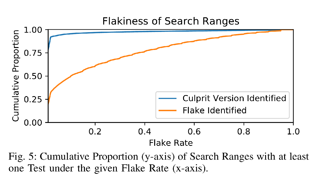
We therefore examine the overall dataset for discrepancies between the two categories. For example, flaky ranges have, on average, 8 tests failing while non-flaky ranges have 224. For the objective of finding unique real culprits, we are interested in the minimum flake rate over targets in a range for flaky and non-flaky ranges, respectively. Fig [fig:min-flake-rate] shows us that, in fact, 99% of real culprit ranges have targets below a flake rate of 75%.

Results

RQ1: Which algorithm (FACF or Bisect) was more accurate in identifying culprit commits?

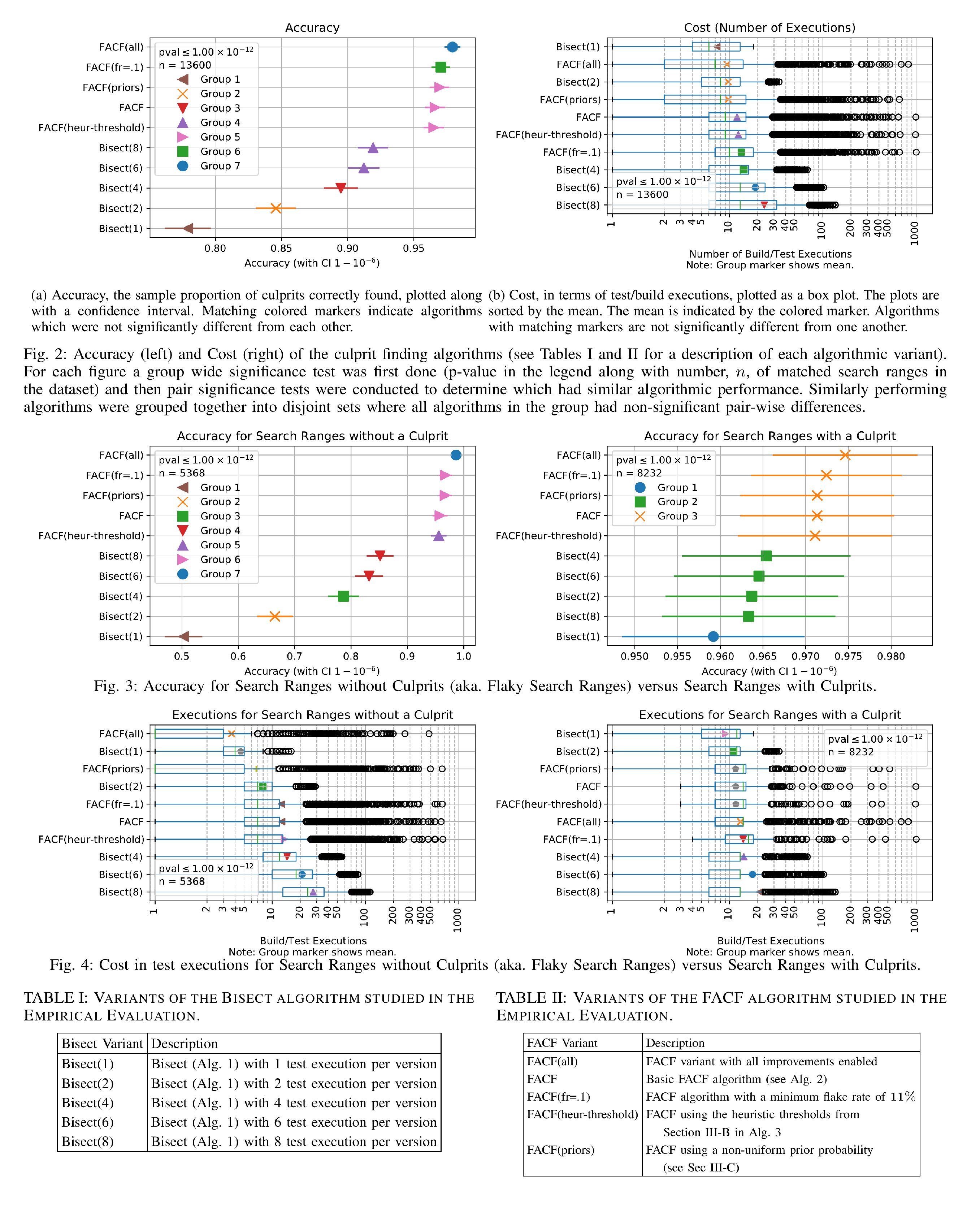
All versions of FACF were more accurate overall than all versions of Bisect (Figure 2). The difference was significant with a p-value \(< 10^{-12}\), below the adjusted \(10^{-6}\) significance level required.

RQ2: What difference do algorithmic tweaks (such as adding deflaking runs to Bisect) make to accuracy?

The production version of FACF, FACF(all), was most accurate and significantly different than all other algorithms (Figure 2). This was followed by FACF(fr=.1) which set the floor of 10% on the estimated flake rate for tests. The other FACF variants were equally accurate.

RQ3: How efficient is each algorithm as measured in number of test executions?

Figure 2 shows the most efficient algorithm was unsurprisingly Bisect(1) which does not attempt to do any extra executions to deflake test failures. The next most efficient algorithm was FACF(all) which was also the most accurate. As can be seen in the boxplot in Figure 2, the FACF variants tend to have many more extreme outliers in their cost distribution than the Bisect variants. This is because they account for the prior flake rate. An organization may control their cost by not culprit finding tests which are more than (for instance) 50% flaky. No such upper bound was established for this experiment.

RQ4: What difference do algorithmic tweaks (such as adding deflaking runs to Bisect) make to efficiency?

First, both FACF(all) and FACF(priors) had less cost than the standard FACF. This indicates that while FACF(priors) does not improve accuracy it does improve efficiency of the algorithm. In particular many more culprits were found with just two builds.

Second, FACF(heur-thresholds) had no significant effect on cost nor did it show any improvement accuracy. We conclude that although the mathematical motivation may be sound, in the Google environment, we cannot validate a benefit to this optimization at this time.

RQ5: Does flakiness affect culprit finding accuracy and cost?

Figures 3 and 4 show the accuracy and cost of culprit finding flaky and non-flaky culprits. For search ranges without a culprit, FACF(all) clearly dominates Bisect in accuracy and even has a small advantage in cost over Bisect(1).

When there is a culprit, the FACF variants are all more accurate than the Bisect variants according to the statistical tests. However, the difference is much less pronounced with Bisect(1) accuracy \(\sim\)96.1% and FACF(all) accuracy \(\sim\)97.5%. In terms of cost, Bisect(1) and Bisect(2) are the most efficient followed by the FACF variants.

We will note, a production culprit finder cannot know a priori if a breakage was caused by a flake. It would need to do deflaking runs to establish that, costing approximately \(\left\lceil{\frac{\,\textrm{log}\!\!\left({p}\right)}{\,\textrm{log}\!\!\left({\hat{f}_t}\right)}}\right\rceil\) where \(p\) is your desired confidence level. For \(p=10^{-4}\) and \(\hat{f} = .2\), this amounts to 6 extra runs, which would significantly increase the cost of bisection. However, as noted in Section 5.5, prior flakiness rates could be used to prune out a significant portion of flaky ranges (lowering cost) with a minimal hit to accuracy.

Related Work

Culprit Finding

Despite its industrial importance, culprit finding has been relatively less studied in the literature in comparison to topics such as Fault Localization (Agarwal and Agrawal 2014; Wong et al. 2016) (coverage based (J. a. Jones, Harrold, and Stasko 2002; J. A. Jones and Harrold 2005; Lucia et al. 2014; Henderson and Podgurski 2018; Henderson, Podgurski, and Kucuk 2019; Kucuk, Henderson, and Podgurski 2021), information retrieval based (J. Zhou, Zhang, and Lo 2012; Youm et al. 2015; Ciborowska and Damevski 2022), or slicing based (Podgurski and Clarke 1990; Horwitz and Reps 1992; Ren et al. 2004)), Bug Prediction (Lewis et al. 2013; Punitha and Chitra 2013; Osman et al. 2017), Test Selection (Engström, Runeson, and Skoglund 2010; Pan et al. 2022), Test Prioritization (de S. Campos Junior et al. 2017; Pan et al. 2022) and the SZZ algorithm for identifying bug inducing commits in the context of research studies (Śliwerski, Zimmermann, and Zeller 2005; Rodríguez-Pérez, Robles, and González-Barahona 2018; Borg et al. 2019; Wen et al. 2019). This is perhaps understandable as the problem only emerges in environments were it becomes to costly to run every test at every code submission.

The idea of using a binary search to locate the culprit is common, but it is not completely clear who invented it first. The Christian Couder of git bisect wrote a comprehensive paper on its implementation (Couder 2008) but indicates there are other similar tools: “So what are the tools used to fight regressions? [...] The only specific tools are test suites and tools similar to git bisect.” The first version of the git bisect command appears to have been written by Linus Torvalds in 2005.⁵ Torvald’s commit message simply states “This is useful for doing binary searching for problems.” The source code for the mercurial bisect command hg bisect states that it was inspired by the git command.⁶ The Subversion (SVN) command, svn bisect, also cites the git command as inspiration.⁷ Therefore, as far as the authors can tell bisection for finding culprits appears to have been invented by Torvalds.

The Couder paper (Couder 2008) cites a GitHub repository for a program called “BBChop,” which is lightly documented and appears not entirely completed by a user enigmatically named Ealdwulf Wuffinga (likely a pseudonym, as that was a name of the King of East Anglia from 664-713).⁸ This program claims to have also implemented a Bayesian search for culprits. We gladly cede the throne for first invention of applying Bayes rule to culprit finding to Ealdwulf and note that our invention was independent of the work in BBChop.

More recently, work has been emerging on the industrial practice of Culprit Finding. In 2013, Ziftci and Ramavajjala gave a public talk at the Google Test Automation Conference in on Culprit Finding at Google (Ziftci and Ramavajjala 2013). They note, that by 2013 Google has already been using \(m\)-ary bisection based culprit finding for “small” and “medium” tests. They then give a preview of an approach elaborated on in Ziftci and Reardon’s 2017 paper (Ziftci and Reardon 2017) for culprit finding integration tests where test executions take a long time to run. The authors propose a suspiciousness metric based on the minimum build dependence distance and conduct a case study on the efficacy of using such a metric to surface potential culprits to developers. We utilize a similar build dependence distance as input to construct a prior probability (see Section 3.3) in this work but do not directly surface the metric to our end users. Finally, for ground truth they rely on the developers to report what the culprit version is. In contrast, the empirical evaluation we present in this new work is fully automated and does not rely on developers.

In 2017, Saha and Gligoric (Saha and Gligoric 2017) proposed accelerating the traditional bisect algorithm via Test Selection techniques. They use Coverage Based Test Selection (Z. Q. Zhou 2010; Musa et al. 2015) to choose which commits are most likely to affect the test results at the failing commit. This technique can be viewed as fine grained, dynamic version of the static build dependence selection strategy we employ at Google.

In 2019, Najafi et al. (Najafi, Rigby, and Shang 2019) looked at a similar problem to the traditional culprit finding problem we examine here. In their scenario, there is a submission queue that queues up commits to integrate into the main development branch. It batches these waiting commits and tests them together. If a test fails, they need to culprit find to determine the culprit commit. The authors evaluate using a ML-driven risk based batching approach. In 2022, the same research group re-evaluated the 2019 paper on an open source dataset in Beheshtian et al.’s 2022 paper (Beheshtian, Bavand, and Rigby 2022). They found that in the new environment the risk based batching didn’t do as well as a new and improved combinatorics based batching scheme for identifying the culprit commits.

James Keenan gave a presentation in 2019 at the Perl Conference in which he presented a concept, multisection, for dealing with multiple bugs in the same search range (Keenan 2019). Ideally, industrial culprit finders would automatically detect that there are multiple distinct bug inducing commits.

In 2021, two papers looked at using coverage based data for accelerating bug localization. An and Yoo (An and Yoo 2021) used coverage data to accelerate both bisection and SZZ (Śliwerski, Zimmermann, and Zeller 2005) and found significant speedups. Wen et al. (Wen et al. 2021) combined traditional Coverage Based Statistical Fault Localization (J. a. Jones, Harrold, and Stasko 2002) with historical information to create a new suspiciousness score (Sun and Podgurski 2016). This fault localization method could be used in a culprit finding context by using the line rankings to rank the commits.

Finally, in 2022 Frolin Ocariza (Ocariza 2022) published a paper on bisecting performance regressions. There are strong connections between a flaky test and a performance regression as a performance regression may not happen 100% of the time. Furthermore, the “baseline” version may randomly have poor performance due to environmental or other factors. Ocariza also arrives at a probabilistic approach, using a Bayesian model to determine whether a run at a particular version is exhibiting the performance regression or not. While mathematically related to our work here and complementary, the approach is distinct. The authors note that their technique can be combined with a Noisy Binary Search citing Karp (Karp and Kleinberg 2007) or with a multisection search citing Keenan (Keenan 2019).

Noisy Binary Search

There is a vast literature on Rényi-Ulam games and Noisy Searching problems (doubly so when considering their connection to error correcting codes)! We direct readers to the Pelc survey (Pelc 2002) as a starting point. We will highlight a few articles here. First and foremost, the Ben Or and Hassidim paper (Ben-Or and Hassidim 2008) from 2008 most clearly explains the problem in terms of a Bayesian inference, which is the formulation we use here. Second, Waeber et al. in 2013 (Waeber, Frazier, and Henderson 2013) discuss the theoretical foundations of these probabilistic bisection algorithms. Finally, according to Waeber, Horstein first described this algorithm in the context of error correcting codes in 1963 (Horstein 1963).

Conclusion

Flake Aware Culprit Finding (FACF) is both accurate, efficient, and able to flexibly incorporate prior information on the location of a culprit. A large scale empirical study on real test and build breakages found FACF to be significantly more effective than a traditional bisection search while not increasing cost over a deflaked bisection.

References

---

1. In practice the restriction on network usage on TAP is somewhat loose. There are legacy tests that have been tagged to allow them to utilize the network and there is an on going effort to fully eliminate network usage on TAP.↩︎

2. Other CI platforms exist for integration tests that span multiple machines, use large amounts of RAM, or take a very long time to run. The algorithm presented in this paper has also been implemented for one of those CI systems but we will not present an empirical evaluation of its performance in that environment in this paper. In general, Culprit Finding is much more difficult in such environments as tests may use a mixture of code from different versions and network resources may be shared across tests.↩︎

3. An internal version of Bazel https://bazel.build/.↩︎

4. The exact number of hours isn’t so important. The main thing is to repeat the verification at a suitable interval from the original attempt.↩︎

5. https://github.com/git/git/commit/8b3a1e056f2107deedfdada86046971c9ad7bb87↩︎

6. https://www.mercurial-scm.org/repo/hg/file/52464a20add0/mercurial/hbisect.py, https://www.mercurial-scm.org/repo/hg/rev/a7678cbd7c28↩︎

7. https://metacpan.org/release/INFINOID/App-SVN-Bisect-1.1/source/README↩︎

8. https://github.com/Ealdwulf/bbchop↩︎

References

- Agarwal, Pragya, and Arun Prakash Agrawal. 2014. “Fault-Localization Techniques for Software Systems: A Literature Review.” SIGSOFT Softw. Eng. Notes 39 (5): 1–8. https://doi.org/10.1145/2659118.2659125.
- An, Gabin, and Shin Yoo. 2021. “Reducing the Search Space of Bug Inducing Commits Using Failure Coverage.” In Proceedings of the 29th ACM Joint Meeting on European Software Engineering Conference and Symposium on the Foundations of Software Engineering, 1459–62. Athens Greece: ACM. https://doi.org/10.1145/3468264.3473129.
- Ananthanarayanan, Sundaram, Masoud Saeida Ardekani, Denis Haenikel, Balaji Varadarajan, Simon Soriano, Dhaval Patel, and Ali Reza Adl-Tabatabai. 2019. “Keeping Master Green at Scale.” Proceedings of the 14th EuroSys Conference 2019. https://doi.org/10.1145/3302424.3303970.
- Beheshtian, Mohammad Javad, Amir Hossein Bavand, and Peter C. Rigby. 2022. “Software Batch Testing to Save Build Test Resources and to Reduce Feedback Time.” IEEE Transactions on Software Engineering 48 (8): 2784–2801. https://doi.org/10.1109/TSE.2021.3070269.
- Ben-Or, Michael, and Avinatan Hassidim. 2008. “The Bayesian Learner Is Optimal for Noisy Binary Search (and Pretty Good for Quantum as Well).” In 2008 49th Annual IEEE Symposium on Foundations of Computer Science, 221–30. Philadelphia, PA, USA: IEEE. https://doi.org/10.1109/FOCS.2008.58.
- Bhattacharya, Pamela, and Iulian Neamtiu. 2010. “Fine-Grained Incremental Learning and Multi-Feature Tossing Graphs to Improve Bug Triaging.” In 2010 IEEE International Conference on Software Maintenance, 1–10. Timi oara, Romania: IEEE. https://doi.org/10.1109/ICSM.2010.5609736.
- Binkley, D. 1992. “Using Semantic Differencing to Reduce the Cost of Regression Testing.” In Proceedings Conference on Software Maintenance 1992, 41–50. Orlando, FL, USA: IEEE Comput. Soc. Press. https://doi.org/10.1109/ICSM.1992.242560.
- Borg, Markus, Oscar Svensson, Kristian Berg, and Daniel Hansson. 2019. “SZZ Unleashed: An Open Implementation of the SZZ Algorithm - Featuring Example Usage in a Study of Just-in-Time Bug Prediction for the Jenkins Project.” In Proceedings of the 3rd ACM SIGSOFT International Workshop on Machine Learning Techniques for Software Quality Evaluation - MaLTeSQuE 2019, 7–12. Tallinn, Estonia: ACM Press. https://doi.org/10.1145/3340482.3342742.
- Ciborowska, Agnieszka, and Kostadin Damevski. 2022. “Fast Changeset-Based Bug Localization with BERT.” In Proceedings of the 44th International Conference on Software Engineering, 946–57. Pittsburgh Pennsylvania: ACM. https://doi.org/10.1145/3510003.3510042.
- Couder, Christian. 2008. “Fighting Regressions with Git Bisect.” The Linux Kernel Archives 4 (5). https://www. kernel. org/pub/software/scm/git/doc s/git- bisect-lk2009.html.
- de S. Campos Junior, Heleno, Marco Antônio P Araújo, José Maria N David, Regina Braga, Fernanda Campos, and Victor Ströele. 2017. “Test Case Prioritization: A Systematic Review and Mapping of the Literature.” In Proceedings of the 31st Brazilian Symposium on Software Engineering, 34–43. New York, NY, USA: ACM. https://doi.org/10.1145/3131151.3131170.
- Engström, Emelie, Per Runeson, and Mats Skoglund. 2010. “A Systematic Review on Regression Test Selection Techniques.” Information and Software Technology 52 (1): 14–30. https://doi.org/10.1016/j.infsof.2009.07.001.
- Fowler, Martin. 2006. “Continuous Integration.” https://martinfowler.com/articles/ continuousIntegration.html.
- Gupta, Pooja, Mark Ivey, and John Penix. 2011. “Testing at the Speed and Scale of Google.” http://google-engtools.blogspot.com/2011/06/testing-at- speed-and-scale-of-google.html.
- Henderson, Tim A. D., and Andy Podgurski. 2018. “Behavioral Fault Localization by Sampling Suspicious Dynamic Control Flow Subgraphs.” In 2018 IEEE 11th International Conference on Software Testing, Verification and Validation (ICST), 93–104. Vasteras: IEEE. https://doi.org/10.1109/ICST.2018.00019.
- Henderson, Tim A. D., Andy Podgurski, and Yigit Kucuk. 2019. “Evaluating Automatic Fault Localization Using Markov Processes.” In 2019 19th International Working Conference on Source Code Analysis and Manipulation (SCAM), 115–26. Cleveland, OH, USA: IEEE. https://doi.org/10.1109/SCAM.2019.00021.
- Herzig, Kim, Michaela Greiler, Jacek Czerwonka, and Brendan Murphy. 2015. “The Art of Testing Less Without Sacrificing Quality.” In 2015 IEEE/ACM 37th IEEE International Conference on Software Engineering, 1:483–93. IEEE. https://doi.org/10.1109/ICSE.2015.66.
- Herzig, Kim, and Nachiappan Nagappan. 2015. “Empirically Detecting False Test Alarms Using Association Rules.” In 2015 IEEE/ACM 37th IEEE International Conference on Software Engineering, 39–48. Florence, Italy: IEEE. https://doi.org/10.1109/ICSE.2015.133.
- Horstein, M. 1963. “Sequential Transmission Using Noiseless Feedback.” IEEE Transactions on Information Theory 9 (3): 136–43. https://doi.org/10.1109/TIT.1963.1057832.
- Horwitz, S, and T Reps. 1992. “The Use of Program Dependence Graphs in Software Engineering.” In International Conference on Software Engineering, 9:349. Springer. http://portal.acm.org/citation.cfm?id=24041&dl=.
- Jones, J.a., M. J. Harrold, and J. Stasko. 2002. “Visualization of Test Information to Assist Fault Localization.” Proceedings of the 24th International Conference on Software Engineering. ICSE 2002. https://doi.org/10.1145/581339.581397.
- Jones, James A., and Mary Jean Harrold. 2005. “Empirical Evaluation of the Tarantula Automatic Fault-localization Technique.” In Proceedings of the 20th IEEE/ACM International Conference on Automated Software Engineering, 273–82. New York, NY, USA: ACM. https://doi.org/10.1145/1101908.1101949.
- Just, René, Darioush Jalali, and Michael D Ernst. 2014. “Defects4J: A Database of Existing Faults to Enable Controlled Testing Studies for Java Programs.” In Proceedings of the 2014 International Symposium on Software Testing and Analysis, 437–40. New York, NY, USA: ACM. https://doi.org/10.1145/2610384.2628055.
- Karp, Richard M., and Robert Kleinberg. 2007. “Noisy Binary Search and Its Applications.” In Proceedings of the Eighteenth Annual ACM-SIAM Symposium on Discrete Algorithms, 881–90. SODA ’07. USA: Society for Industrial and Applied Mathematics. https://dl.acm.org/doi/abs/10.5555/1283383.1283478.
- Keenan, James. 2019. “James E. Keenan - "Multisection: When Bisection Isn’t Enough to Debug a Problem".” https://www.youtube.com/watch?v=05CwdTRt6AM.
- Kowalczyk, Emily, Karan Nair, Zebao Gao, Leo Silberstein, Teng Long, and Atif Memon. 2020. “Modeling and Ranking Flaky Tests at Apple.” In Proceedings of the ACM/IEEE 42nd International Conference on Software Engineering: Software Engineering in Practice, 110–19. Seoul South Korea: ACM. https://doi.org/10.1145/3377813.3381370.
- Kucuk, Yigit, Tim A. D. Henderson, and Andy Podgurski. 2021. “Improving Fault Localization by Integrating Value and Predicate Based Causal Inference Techniques.” In 2021 IEEE/ACM 43rd International Conference on Software Engineering (ICSE), 649–60. Madrid, ES: IEEE. https://doi.org/10.1109/ICSE43902.2021.00066.
- Leong, Claire, Abhayendra Singh, Mike Papadakis, Yves Le Traon, and John Micco. 2019. “Assessing Transition-Based Test Selection Algorithms at Google.” In 2019 IEEE/ACM 41st International Conference on Software Engineering: Software Engineering in Practice (ICSE-SEIP), 101–10. IEEE. https://doi.org/10.1109/ICSE-SEIP.2019.00019.
- Lewis, Chris, Zhongpeng Lin, Caitlin Sadowski, and Xiaoyan Zhu. 2013. “Does Bug Prediction Support Human Developers? Findings from a Google Case Study.” In Proceedings of the …, 372–81. http://dl.acm.org/citation.cfm?id=2486838.
- Lucia, David Lo, Lingxiao Jiang, Ferdian Thung, and Aditya Budi. 2014. “Extended Comprehensive Study of Association Measures for Fault Localization.” Journal of Software: Evolution and Process 26 (2): 172–219. https://doi.org/10.1002/smr.1616.
- Machalica, Mateusz, Wojtek Chmiel, Stanislaw Swierc, and Ruslan Sakevych. 2020. “Probabilistic Flakiness: How Do You Test Your Tests?” DEVINFRA. https://engineering.fb.com/2020/12/10/developer-tools/ probabilistic-flakiness/.
- Machalica, Mateusz, Alex Samylkin, Meredith Porth, and Satish Chandra. 2019. “Predictive Test Selection.” In 2019 IEEE/ACM 41st International Conference on Software Engineering: Software Engineering in Practice (ICSE-SEIP), 91–100. IEEE. https://doi.org/10.1109/ICSE-SEIP.2019.00018.
- McCrum-Gardner, Evie. 2008. “Which Is the Correct Statistical Test to Use?” British Journal of Oral and Maxillofacial Surgery 46 (1): 38–41. https://doi.org/10.1016/j.bjoms.2007.09.002.
- Memon, Atif, Zebao Gao, Bao Nguyen, Sanjeev Dhanda, Eric Nickell, Rob Siemborski, and John Micco. 2017. “Taming Google-scale Continuous Testing.” In 2017 IEEE/ACM 39th International Conference on Software Engineering: Software Engineering in Practice Track (ICSE-SEIP), 233–42. Piscataway, NJ, USA: IEEE. https://doi.org/10.1109/ICSE-SEIP.2017.16.
- Micco, John. 2012. “Tools for Continuous Integration at Google Scale.” Tech {{Talk}}. Google NYC. https://youtu.be/KH2_sB1A6lA.
- ———. 2013. “Continuous Integration at Google Scale.” Lecture. EclipseCon 2013. https://web.archive.org/web/20140705215747/https:// www.eclipsecon.org/2013/sites/eclipsecon.org.2013/files/2013- 03-24%20Continuous%20Integration%20at%20Google%20Scale.pdf.
- Musa, Samaila, Abu Bakar Md Sultan, Abdul Azim Bin Abd-Ghani, and Salmi Baharom. 2015. “Regression Test Cases Selection for Object-Oriented Programs Based on Affected Statements.” International Journal of Software Engineering and Its Applications 9 (10): 91–108. https://doi.org/10.14257/ijseia.2015.9.10.10.
- Najafi, Armin, Peter C. Rigby, and Weiyi Shang. 2019. “Bisecting Commits and Modeling Commit Risk During Testing.” In Proceedings of the 2019 27th ACM Joint Meeting on European Software Engineering Conference and Symposium on the Foundations of Software Engineering, 279–89. New York, NY, USA: ACM. https://doi.org/10.1145/3338906.3338944.
- Ocariza, Frolin S. 2022. “On the Effectiveness of Bisection in Performance Regression Localization.” Empirical Software Engineering 27 (4): 95. https://doi.org/10.1007/s10664-022-10152-3.
- Osman, Haidar, Mohammad Ghafari, Oscar Nierstrasz, and Mircea Lungu. 2017. “An Extensive Analysis of Efficient Bug Prediction Configurations.” In Proceedings of the 13th International Conference on Predictive Models and Data Analytics in Software Engineering, 107–16. Toronto Canada: ACM. https://doi.org/10.1145/3127005.3127017.
- Pan, Rongqi, Mojtaba Bagherzadeh, Taher A. Ghaleb, and Lionel Briand. 2022. “Test Case Selection and Prioritization Using Machine Learning: A Systematic Literature Review.” Empirical Software Engineering 27 (2): 29. https://doi.org/10.1007/s10664-021-10066-6.
- Pelc, Andrzej. 2002. “Searching Games with Errorsfifty Years of Coping with Liars.” Theoretical Computer Science 270 (1-2): 71–109. https://doi.org/10.1016/S0304-3975(01)00303-6.
- Podgurski, A, and L A Clarke. 1990. “A Formal Model of Program Dependences and Its Implications for Software Testing, Debugging, and Maintenance.” IEEE Transactions of Software Engineering 16 (9): 965–79. https://doi.org/10.1109/32.58784.
- Potvin, Rachel, and Josh Levenberg. 2016. “Why Google Stores Billions of Lines of Code in a Single Repository.” Communications of the ACM 59 (7): 78–87. https://doi.org/10.1145/2854146.
- Punitha, K., and S. Chitra. 2013. “Software Defect Prediction Using Software Metrics - A Survey.” In 2013 International Conference on Information Communication and Embedded Systems (ICICES), 555–58. Chennai: IEEE. https://doi.org/10.1109/ICICES.2013.6508369.
- Ren, Xiaoxia, Fenil Shah, Frank Tip, Barbara G. Ryder, and Ophelia Chesley. 2004. “Chianti: A Tool for Change Impact Analysis of Java Programs.” In Proceedings of the 19th Annual ACM SIGPLAN Conference on Object-oriented Programming, Systems, Languages, and Applications, 432–48. Vancouver BC Canada: ACM. https://doi.org/10.1145/1028976.1029012.
- Rivest, R. L., A. R. Meyer, and D. J. Kleitman. 1978. “Coping with Errors in Binary Search Procedures (Preliminary Report).” In Proceedings of the Tenth Annual ACM Symposium on Theory of Computing - STOC ’78, 227–32. San Diego, California, United States: ACM Press. https://doi.org/10.1145/800133.804351.
- Rodríguez-Pérez, Gema, Gregorio Robles, and Jesús M. González-Barahona. 2018. “Reproducibility and Credibility in Empirical Software Engineering: A Case Study Based on a Systematic Literature Review of the Use of the SZZ Algorithm.” Information and Software Technology 99 (July): 164–76. https://doi.org/10.1016/j.infsof.2018.03.009.
- Saha, Ripon, and Milos Gligoric. 2017. “Selective Bisection Debugging.” In Fundamental Approaches to Software Engineering, edited by Marieke Huisman and Julia Rubin, 10202:60–77. Berlin, Heidelberg: Springer Berlin Heidelberg. https://doi.org/10.1007/978-3-662-54494-5_4.
- Śliwerski, Jacek, Thomas Zimmermann, and Andreas Zeller. 2005. “When Do Changes Induce Fixes?” ACM SIGSOFT Software Engineering Notes 30 (4): 1. https://doi.org/10.1145/1082983.1083147.
- Sun, Shih-Feng, and Andy Podgurski. 2016. “Properties of Effective Metrics for Coverage-Based Statistical Fault Localization.” In 2016 IEEE International Conference on Software Testing, Verification and Validation (ICST), 124–34. IEEE. https://doi.org/10.1109/ICST.2016.31.
- Tharwat, Alaa. 2021. “Classification Assessment Methods.” Applied Computing and Informatics 17 (1): 168–92. https://doi.org/10.1016/j.aci.2018.08.003.
- Tip, Frank. 1995. “A Survey of Program Slicing Techniques.” Journal of Programming Languages 3 (3): 121–89.
- Waeber, Rolf, Peter I. Frazier, and Shane G. Henderson. 2013. “Bisection Search with Noisy Responses.” SIAM Journal on Control and Optimization 51 (3): 2261–79. https://doi.org/10.1137/120861898.
- Walpole, Ronald E., ed. 2007. Probability & Statistics for Engineers & Scientists. 8th ed. Upper Saddle River, NJ: Pearson Prentice Hall.
- Wang, Kaiyuan, Greg Tener, Vijay Gullapalli, Xin Huang, Ahmed Gad, and Daniel Rall. 2020. “Scalable Build Service System with Smart Scheduling Service.” In Proceedings of the 29th ACM SIGSOFT International Symposium on Software Testing and Analysis, 452–62. Virtual Event USA: ACM. https://doi.org/10.1145/3395363.3397371.
- Wen, Ming, Junjie Chen, Yongqiang Tian, Rongxin Wu, Dan Hao, Shi Han, and Shing-Chi Cheung. 2021. “Historical Spectrum Based Fault Localization.” IEEE Transactions on Software Engineering 47 (11): 2348–68. https://doi.org/10.1109/TSE.2019.2948158.
- Wen, Ming, Rongxin Wu, Yepang Liu, Yongqiang Tian, Xuan Xie, Shing-Chi Cheung, and Zhendong Su. 2019. “Exploring and Exploiting the Correlations Between Bug-Inducing and Bug-Fixing Commits.” In Proceedings of the 2019 27th ACM Joint Meeting on European Software Engineering Conference and Symposium on the Foundations of Software Engineering, 326–37. Tallinn Estonia: ACM. https://doi.org/10.1145/3338906.3338962.
- Wong, W. Eric, Ruizhi Gao, Yihao Li, Rui Abreu, and Franz Wotawa. 2016. “A Survey on Software Fault Localization.” IEEE Transactions on Software Engineering 42 (8): 707–40. https://doi.org/10.1109/TSE.2016.2521368.
- Youm, Klaus Changsun, June Ahn, Jeongho Kim, and Eunseok Lee. 2015. “Bug Localization Based on Code Change Histories and Bug Reports.” In 2015 Asia-Pacific Software Engineering Conference (APSEC), 190–97. New Delhi: IEEE. https://doi.org/10.1109/APSEC.2015.23.
- Zhou, Jian, Hongyu Zhang, and David Lo. 2012. “Where Should the Bugs Be Fixed? More Accurate Information Retrieval-Based Bug Localization Based on Bug Reports.” Proceedings - International Conference on Software Engineering, 14–24. https://doi.org/10.1109/ICSE.2012.6227210.
- Zhou, Zhi Quan. 2010. “Using Coverage Information to Guide Test Case Selection in Adaptive Random Testing.” Proceedings - International Computer Software and Applications Conference, 208–13. https://doi.org/10.1109/COMPSACW.2010.43.
- Ziftci, Celal, and Vivek Ramavajjala. 2013. “Finding Culprits Automatically in Failing Builds - i.e. Who Broke the Build?” https://www.youtube.com/watch?v=SZLuBYlq3OM.
- Ziftci, Celal, and Jim Reardon. 2017. “Who Broke the Build? Automatically Identifying Changes That Induce Test Failures in Continuous Integration at Google Scale.” Proceedings - 2017 IEEE/ACM 39th International Conference on Software Engineering: Software Engineering in Practice Track, ICSE-SEIP 2017, 113–22. https://doi.org/10.1109/ICSE-SEIP.2017.13.