Faster Tokenization with a DFA Backend for Lexmachine
Lexmachine is a lexical analysis (or tokenization) library for Go (golang) and it just got faster thanks to a new backend I wrote. This article is going to explain the new backend, how it works, and why it is faster. If you want to use lexmachine checkout the documentation or the tutorial.
Lexical analysis is the process of breaking strings up into substrings, called
lexemes, and putting them into categories called tokens. This process is
also called tokenization and is the first step in parsing complex file
formats, programming languages, network protocols, and other information. Let's
look at a quick example, suppose we wanted to process a custom configuration
file format. For instance,
sensors.conf describes how Linux
should translate the raw readings hardware monitoring chips to real-world values
-- such as voltage and temperature. The first part of my laptop's sensors.conf
file begins with the following:
# It is recommended not to modify this file, but to drop your local
# changes in /etc/sensors.d/. File with names that start with a dot
# are ignored.

chip "lm78-*" "lm79-*" "lm80-*" "lm96080-*"

    label temp1 "M/B Temp"


chip "w83792d-*"

    label in0 "VcoreA"
    label in1 "VcoreB"
    label in6 "+5V"
    label in7 "5VSB"
    label in8 "Vbat"

    set in6_min  5.0 * 0.90
    set in6_max  5.0 * 1.10
    set in7_min  5.0 * 0.90
    set in7_max  5.0 * 1.10
    set in8_min  3.0 * 0.90
    set in8_max  3.0 * 1.10
According to the man page, there are
several syntactic elements in this file: keywords (chip, label, set, ...),
names (in0, in6_min, ..., "lm78-*", "VcoreA", ...), floats (5.0,
0.90, ...), operators (+, -, *, ...), and comments which start with #.
A lexical analysis would break down the file as follows:
Type    | Lexeme
-------------------
COMMENT | # It is recommended not to modify this file, but to drop your local
COMMENT | # changes in /etc/sensors.d/. File with names that start with a dot
COMMENT | # are ignored.
CHIP    | chip
NAME    | "lm78-*"
NAME    | "lm78-*"
NAME    | "lm79-*"
NAME    | "lm80-*"
NAME    | "lm96080-*"
LABEL   | label
NAME    | temp1
NAME    | "M/B Temp"
CHIP    | chip
NAME    | "w83792d-*"
...
SET     | set
NAME    | in8_max
FLOAT   | 3.0
STAR    | *
FLOAT   | 1.10
The categories are defined by patterns which are expressed as regular
expressions. As a
quick review, regular expressions (regex) are a "pattern" which describe a set
of strings. A regex is made up of characters (a, b, 0, @, ...) which
combine with the operators: concatenation abc, alternation a|b, grouping
a(b|c)d, and repetition a*. Some examples:
abcmatches {"abc"}a|bmatches {"a","b"}a(b|c)dmatches {"abd","acd"}a*matches {"","a","aa", ...}a(b(c|d))*matches {"a","abc","abd","abcbc","abcbd", ...}
In the running example of the sensors.conf file one might define the following
patterns:
- AT:
@ - PLUS:
+ - STAR:
* - DASH:
- - SLASH:
/ - CARROT:
^ - BACKTICK:
` - LPAREN:
( - RPAREN:
) - BUS:
bus - CHIP:
chip - LABEL:
label - COMPUTE:
compute - IGNORE:
ignore - SET:
set - NUMBER:
[0-9]*\.?[0-9]+ - NAME:
[a-zA-Z_][a-zA-Z0-9_]*|"[^"]*"
These patterns define how text in the input should categorized according to the
rules for the sensors.conf file.
Efficiently Categorizing Substrings with Automata
Now we turn our attention from what lexical analysis is to how it works. Specifically we are going to concern ourselves with the following matters:
- How the lexical analysis problem is different than the one solved by standard implementations of regular expression engines (such as the regexp standard library package).
- How to solve the lexical analysis problem with non-deterministic finite automatons (NFA).
- How deterministic automatons (DFAs) improve on the solution presented by NFAs
The Lexical Analysis Problem
The regular expression problem decides whether a pattern (as specified by a regular expression) matches a given string. If the pattern does describe the string a regular expression engine will answer: yes it matches. Otherwise, it answers: no it does not.
The lexical analysis problem on the other hand seeks to break up (tokenize) a long piece of text based on an ordered set of regular expressions. It does this by proceeding from the start of the string and finding the longest prefix of the string that matches at least one pattern. It then chooses a matching pattern with the highest precedence and outputs the matched text (lexeme) and the category the pattern defines (token type). Solving the lexical analysis problem with a standard regular expression engine is possible but not efficient. With a standard regex engine, the whole piece of text has to be repeatedly scanned for each token to decide on the longest prefix match and highest precedence token type to use.
However, we can use the theory that is used to implement efficient regular expression engines to implement efficient lexical analysis engines. The following adjustments must be made:
- Prefixes of a string are matched
- Several patterns are matched at once
- The pattern which matches the longest prefix wins
- In case of ties, the pattern with the highest precedence wins
Finite Automata
Efficient regular expression engines are implemented using the theory of finite automata. Automata or automatons are theoretical mathematical constructs which specify a machine. Specifically, a machine that reads a string, character by character, and decides whether it is in some language or not (see Figure 1). The language is a type of formal language called a regular language or a Type-3 language in the Chomsky Formal Language Hierarchy.
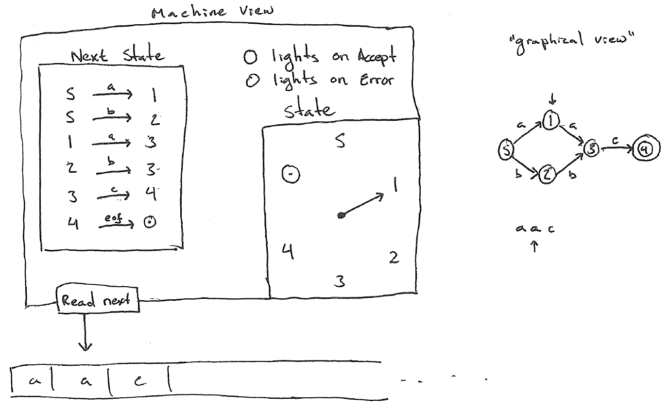
If the string matches the Accept light lights up, otherwise the error light lights up.
Finite state automatons encode their matching "program" as a set of states \(S\), an alphabet \(\Sigma\), and a transition function which maps the current state and next symbol to the next state \( T: S \times \Sigma \rightarrow S \). There are several distinguished states: the starting state, and one or more accepting states. At each step through the input string the machine reads a character and consults the transition function to determine the next state. If at the end of the string the state has reached an accepting state the string is said to match the automaton.
When the transition function \(T\) produces multiple
states for the same input combination the automaton is said to be
non-deterministic. Figure 2 shows a non-deterministic finite automaton
(NFA) for our running example for sensors.conf. In the figure,
the starting state (state 0) may transition on character c
to states 12, 21, and 40. This may be interpreted as the machine transitioning
to all of these states simultaneously and maintaining multiple threads of
execution. Simulations of NFAs must keep track of each independent thread of
execution. If an NFA has \(n\) states and a string
has \(m\) characters it can be matched in \(\mathcal{O}(n \cdot m)\) steps.
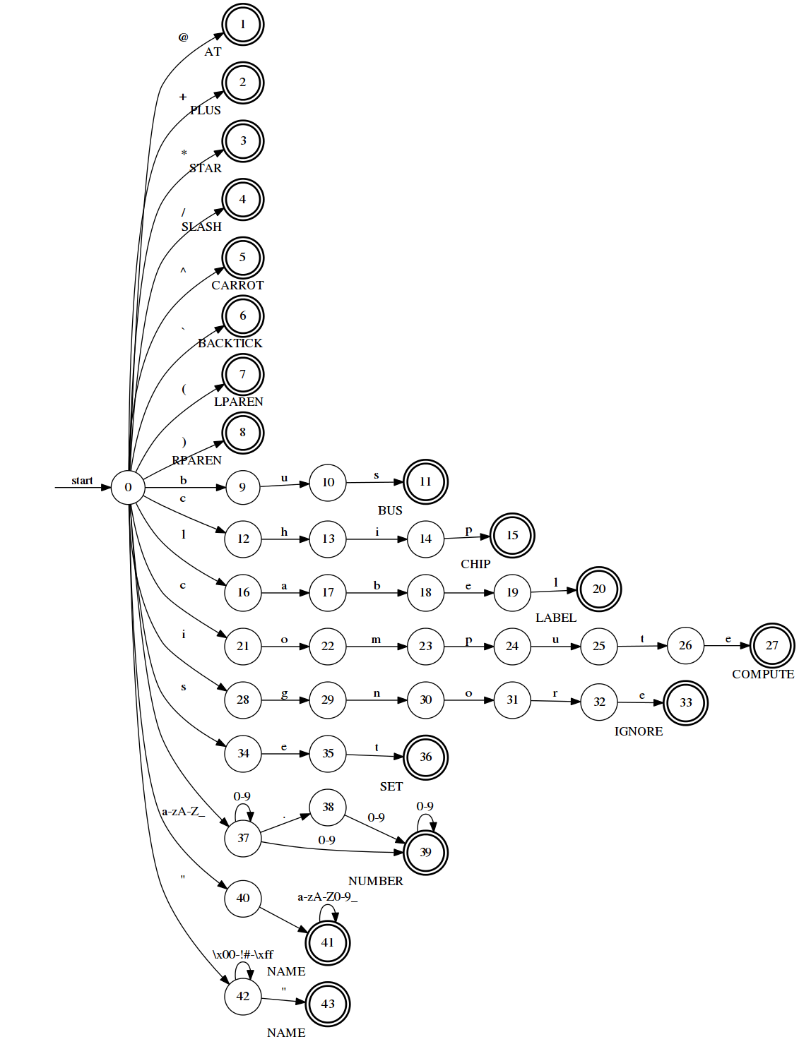
sensors.conf.States with double circles are accepting states. Each accepting state is labeled with the category it corresponds to. The starting state is marked.
To use an NFA for the lexical analysis problem several adjustments need to be made.
- To match prefixes, keep scanning until no new states are found (that is all threads of execution have either reached end of the string or the error state).
- Track all accepting states reached during the scanning.
- Return the "most relevant" match on state exhaustion by returning the accepting state which matched the longest prefix. Ties are broken by user supplied precedence.
- When the user requests the next token, reset the simulation to the starting state and rerun starting at the next character after the previously returned prefix.
- After all input has been consumed check all of the input was successfully matched. Return an error otherwise.
As languages get more complex the cost of tokenization goes up when using NFAs because the cost for matching a regular expression is dependent in the size of the NFA (\(\mathcal{O}(n \cdot m)\) where \(n\) is the number of states in the NFA and \(m\) is the length of the string). Can we do better? We can! If we do not allow the transition function \(T\) to produce more than one state for each input combination the automaton will be deterministic finite automaton (DFA). If the automaton is deterministic then simulation is greatly simplified versus a non-deterministic automaton. Recall, in the case of NFA simulation non-deterministic steps are modeled by having the machine transition to all possible next states at once and keeping track of multiple threads of execution. In a DFA, there will always be one (and only one) state to transition to -- and therefore only one thread of execution. If there is only one thread of execution the simulation can be run in \(\mathcal{O}(m)\) steps (where \(m\) is the length of string).
Figure 3 shows the minimal DFA for the NFA given in Figure 2. By coincidence there is one fewer states in the DFA than in the NFA. In general, this will not be the case. Indeed, in the worst case if the NFA has \(n\) states the DFA could have as many as \(2^{n}\) states. However, on average the DFA will only have \(n^3\) states. Thus, a DFA makes the classic space vs. time tradeoff. It uses more space (in the form of a larger transition table on average) to get faster execution time.
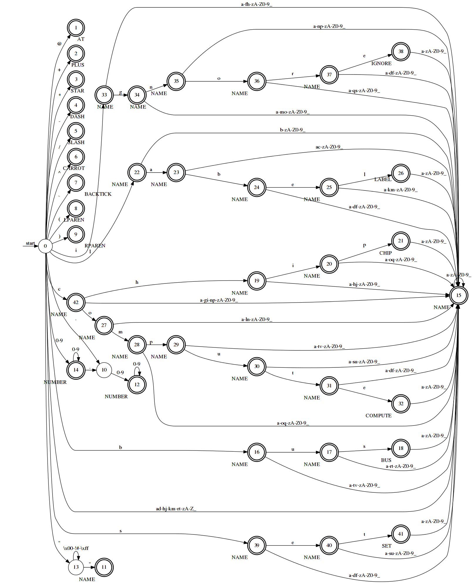
sensors.conf.States with double circles are accepting states. Each accepting state is labeled with the category it corresponds to. The starting state is marked.
Practical Results
Does the new DFA backend outperform the NFA backend when tokenizing many
strings? The answer is yes. As an quick (non-rigorous) example, let's tokenize
my sensors.conf file 1000 times using both the NFA backend and the DFA backend.
Using the NFA backend
$ go install github.com/timtadh/lexmachine/examples/sensors &&
> cat /etc/sensors*.conf | (/usr/bin/time -v sensors --nfa )
        Command being timed: "sensors --nfa"
        User time (seconds): 3.0
        System time (seconds): 0.00
        Percent of CPU this job got: 102%
        Elapsed (wall clock) time (h:mm:ss or m:ss): 0:02.97
        Average shared text size (kbytes): 0
        Average unshared data size (kbytes): 0
        Average stack size (kbytes): 0
        Average total size (kbytes): 0
        Maximum resident set size (kbytes): 6564
        Average resident set size (kbytes): 0
        Major (requiring I/O) page faults: 0
        Minor (reclaiming a frame) page faults: 1749
        Voluntary context switches: 1866
        Involuntary context switches: 473
        Swaps: 0
        File system inputs: 0
        File system outputs: 0
        Socket messages sent: 0
        Socket messages received: 0
        Signals delivered: 0
        Page size (bytes): 4096
        Exit status: 0
Using the DFA backend
$ go install github.com/timtadh/lexmachine/examples/sensors &&
> cat /etc/sensors*.conf | (/usr/bin/time -v sensors --dfa )
        Command being timed: "sensors --dfa"
        User time (seconds): 2.01
        System time (seconds): 0.00
        Percent of CPU this job got: 104%
        Elapsed (wall clock) time (h:mm:ss or m:ss): 0:01.93
        Average shared text size (kbytes): 0
        Average unshared data size (kbytes): 0
        Average stack size (kbytes): 0
        Average total size (kbytes): 0
        Maximum resident set size (kbytes): 7680
        Average resident set size (kbytes): 0
        Major (requiring I/O) page faults: 0
        Minor (reclaiming a frame) page faults: 2172
        Voluntary context switches: 2231
        Involuntary context switches: 359
        Swaps: 0
        File system inputs: 0
        File system outputs: 0
        Socket messages sent: 0
        Socket messages received: 0
        Signals delivered: 0
        Page size (bytes): 4096
        Exit status: 0
Note as predicted by the theory presented above, the NFA backend used less memory but took longer to tokenize the file 1000 times. The DFA backend used more memory (but not a lot more) and tokenized the file faster than the NFA backend.
Intrigued? Try out lexmachine today!